Exercise 1
When can a general \(n\)th order differential equation be cast as a system of \(n\) first-order equations? Give an example of a second order equation that cannot be written this way.
For problems 2-8, recast the given higher-order differential equation into a system of an appropriate number of first-order equations.
Exercise 2
\(y'' + 3y' + 7 = 0\)
Exercise 3
\(y''' + yy'' = 3y^2\sin(y')\)
Exercise 4
\(y^{(5)} = \tan(2t) + 3\)
Exercise 5
\(ty''' + (y')^2 = ye^t + te^y\)
Exercise 6
\(y^{\prime\prime\prime} + y^2y^\prime + 3y = t^2e^{-5t}\)
Exercise 7
\(x^{\prime\prime} + 3x^\prime - ax = 0\)
Exercise 8
\(v^{(4)} + \cos{(v^{\prime\prime})}v - v^\prime v + (v^{\prime\prime\prime})^3 = 0\)
For problems 9-11, recast the initial value problems into initial value problems for a system of first order equations.
Exercise 9
\(u^{(4)} = 0\), \(u(0) = 4\), \(u^\prime(0) = 0\), \(u^{\prime\prime}(0) = -5\), \(u^{\prime\prime\prime}(0) = 0\)
Exercise 10
\(y'' + 3ty = \cos(4t)\), \(y(1) = 2\), \(y^\prime(1) = -2\)
Exercise 11
\(y^{(5)} + \frac{2}{y} = t\), \(y(1) = 0\), \(y^\prime(1) = -1\), \(y^{\prime\prime}(1) = 3\), \(y^{\prime\prime\prime}(1) = -7\), \(y^{\prime\prime\prime\prime}(1) = 2\)
For problems 12-14, recast the systems of higher-order differential equations as first order systems of differential equations.
Exercise 12
\[\begin{split} u^{\prime\prime\prime} &= u + v\\ v^{\prime\prime} &= 2tuv^\prime - v + t\sin{t} \end{split}\]
Exercise 13
\[\begin{split} x^{\prime\prime} &= 4(y-z) + ty^\prime - \sin{(2t)}\\ y^{\prime} &= y + zz^{\prime}\\ z^{\prime\prime} &= 2y + 16x^\prime y - 10yx \end{split}\]
Exercise 14
\[\begin{split} x^{\prime\prime\prime} &= ty^\prime - 3y + x^2e^{3t}\\ y^{\prime\prime} &= 6xy - 2. \end{split}\] With initial conditions \[\begin{split} &x(-2) = 0,\quad x^\prime(-2) = 3,\quad x^{\prime\prime}(-2) = -1,\\ &y(-2) = 8, \quad y^\prime(-2) = 4. \end{split}\]
Exercise 15
Consider two interconnected tanks filled with brine (salt water). The first tank contains 60 liters and the second tank contains 90 liters. Brine with a concentration of 9 grams of salt per liter flows into the first tank at a rate of 6 liters per hour, from the second tank into the first tank at a rate of 3 liters per hour, from the first tank into a drain at a rate of 4 liters per hour, and from the second tank into a drain at a rate of 2 liters per hour. At \(t=0\) there are 90 grams of salt in the first tank and 30 grams of salt in the second tank. Assume that the solution flows between the tanks in such a way that the volumes of the tanks remain constant. Give (but don’t solve) an initial value problem that governs the amount of salt in each tank as a function of time.
Exercise 16
A factory has a pair of interconnected tanks as part of a manufacturing process. The tanks contain a fluid (more of a sludge, but let’s be generous) that has important chemicals in it for whatever it is they’re manufacturing, but we’re interested in the quantity of salt in the tanks because too much salt in the sludge can damage the equipment. The volume of the first tank is \(50\) liters and the volume of the second tank is \(30\) liters; both tanks are full of fluid when the machine is initially turned on. The initial amount of salt in the first tank is \(120\) grams, and initially there are \(64\) grams of salt in the second tank. After the machine is turned on, the well-mixed fluid flows from the first tank to the second one at a rate of \(10\) liters per hour, and in a separate pipe from the second tank back to the first one at a rate of \(3\) liters per hour. The second tank has a drain that leads to the rest of the manufacturing process, and fluid flows down the drain at a rate of \(7\) liters per hour. Fresh sludge is put back into the first tank at a rate of \(7\) liters per hour, and in that fresh sludge there is a salt concentration of \(4\) grams per liter. Write down an initial value problem that governs the amount of salt in each tank as a function of time.
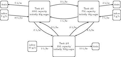
Exercise 17
The following is a schematic for a system of three interconnected tanks with sugar water flowing between them in rates as listed. Write down a initial-value problem that describes how much sugar is in each tank as a function of time.
Exercise 18
Use Euler’s method with two steps to estimate where the solution to the differential equation \[\frac{\dee}{\dt} \begin{pmatrix} x \\ y \end{pmatrix} = \begin{pmatrix} x^2 + ty \\ x + y^2 \end{pmatrix},\] with initial conditions \(x(0) = 1\), \(y(0) = 2\) will be at time \(t=1\).
Exercise 19
Use Runge’s Trapezoidal method with on step to estimate the value of the following system of differential equations at \(t=.5\): \[\frac{\dee}{\dt} \begin{pmatrix} x \\ y \\z \end{pmatrix} = \begin{pmatrix} 3x - z \\ tx + y - 3z \\ t^2(x-z) + 1\end{pmatrix},\] with initial conditions \(x(0) = 1\), \(y(0) = 1\), \(z(0) = 0\).
Exercise 20
Use MATLAB and ode45 to determine where the solution to the initial value problem \[\left\{ \begin{aligned}
\frac{\dee x}{\dee t} & = -2x + 3y \\
\frac{\dee y}{\dee t} & = 3x - 2y \,, \end{aligned} \right.
\hspace{0.4in}
\begin{pmatrix} x(0) = -1 \\ y(0) = 0 \end{pmatrix}\] is at time \(t=5\). Repeat this for the initial conditions \(x(0) = 2\), \(y(0) = 2\).
Exercise 21
This problem uses MATLAB’s command ode45 to investigate the system of differential equations \[\left\{ \begin{aligned}
\frac{\dee x}{\dee t} & = y \\
\frac{\dee y}{\dee t} & = - y - \sin(x)
\end{aligned} \right.\] with initial conditions that are nearby.
Take as initial conditions at time \(t=0\) the point \((x,y) = (0.5,3.75)\). Where does the solution wind up after \(20\) seconds?
Repeat the process but use as initial conditions \((x,y) = (0.5,3.8)\). (You should notice that the two solutions have headed in different directions despite starting close to each other.)
Graph the results of the previous two parts against each other to see where and how they diverge.
Exercise 22
Consider a system of two differential equations \(\frac{\dee \xBld}{\dee t} = \fBld(t,\xBld)\), with \[\xBld = \begin{pmatrix} x_1 \\ x_2 \end{pmatrix} \,, \qquad \fBld(t,\xBld) = \begin{pmatrix} f_1(t, x_1, x_2) \\ f_2(t, x_1, x_2) \end{pmatrix} \,.\] Suppose further that the function \(\fBld\) is continuous, differentiable with respect to each \(x_i\) everywhere, and all its partial derivatives are continuous on \(\R^3\). Suppose also that \[\aBld = (a_1(t, x_1, x_2), a_2(t, x_1, x_2)) \text{ and } \bBld = (b_1(t, x_1, x_2), b_2(t, x_1, x_2)),\] are two different solutions to the system, corresponding to the initial conditions \(\aBld(0) = (0, 0)\) and \(\bBld(0) = (0, 1)\). The functions \(\aBld\) and \(\bBld\) can be viewed as parametrizing curves in the plane. For instance representing the trajectories of particles in two dimensional space. Which of the following statements are true?
The particles could potentially collide, i.e., there can exist a time \(t_c\) with \(\aBld(t_c) = \bBld(t_c)\). (In this case both particles are in the same place at the same time.)
The paths of the particles could potentially cross, i.e., there can exist times \(t_a\) and \(t_b\) with \(\aBld(t_a)=\bBld(t_b)\), but \(t_a\) is not necessarily equal to \(t_b\). (In this case both particles pass through the same place, but at different times.)