The Justin Guide to Matlab for MATH 241 Part 1.
The basic format of this guide is that you will sit down with this page open and a Matlab window open and you will try the guide as you go. Once you are finished following through the guide the project should be very easy.
Contents
Running Matlab
The easiest way to run Matlab is to find a lab on campus and run it there. You can also buy it (expensive!) or the other option is to run it from the Engineering Department's Virtual Lab. You can access that here from the following link. It takes some fiddling (you have to install something called Citrix in order to access the Lab's programs) but most of the people in my Matlab course got this method working so it can't be that bad.
Okay, I'm running Matlab, now what?
When you run Matlab you will see a bunch of windows. The important one will have a prompt in it which looks like >>. This is where we will tell Matlab what to do.
Go into this window and type 2+3. You will see:
2+3
ans =

     5
Oh yeah, you know Matlab! Let's do something more relevant to calculus like take a derivative. Before we do that it's important to note that Matlab works a lot with what are called symbolic expressions. If we want to take a derivative we use the diff command. It's tempting to do diff(x^2) but this errors. Try it and see!
Why does it error? The reason is that Matlab doesn't know what x is and we must tell it that x is a symbol to work with. We do so with the syms command. So we can do the following two commands. The first line tells Matlab that x is symoblic and will be symbolic until we tell it otherwise.
syms x
diff(x^2)
ans =

2*x
Eat your heart out Newton and Leibniz! Here's an even uglier derivative. Keep in mind that we don't need a syms x now because x is still symbolic and will remain so. Notice something important - that multiplication in Matlab always needs a *. Leaving this out will give an error.
diff(2*x^2*sin(x)/cos(x))
ans =

2*x^2 + (2*x^2*sin(x)^2)/cos(x)^2 + (4*x*sin(x))/cos(x)
Oh boy, that's pretty messy. Can we simplify that at all? Indeed we can. We can wrap it in the Matlab command simplify as follows:
simplify(2*diff(x^2*sin(x)/cos(x)))
ans =

2*x^2*tan(x)^2 + 2*x^2 + 4*x*tan(x)
Precalculus
Here are some precalculus things done in Matlab.
Factor a polynomial:
factor(x^4-3*x^3-8*x^2+21*x+9)
ans =

(x^2 + 3*x + 1)*(x - 3)^2
Solve an equation. Notice that we give it a symbolic expression and the solve command assumes that it equals 0 when it solves.
solve(x^2+x-1)
ans =

 - 5^(1/2)/2 - 1/2
   5^(1/2)/2 - 1/2
We can tell it to equal something else but then we have to put the expression in apostrophes. This is sort of annoying.
solve('x^2+x-1=1')
ans =

 -2
  1
Substitute a value into a symbolic expression. Here we tell Matlab to put -1 in place of x. The reason it knows to put it in place of x is that x is the only variable. We'll do some stuff with multiple variables later.
subs(x^3+4/x+1,-1)
ans =

    -4
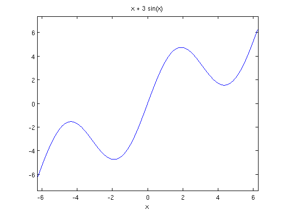
Plot a function. There are many ways to plot in Matlab but the easiest way has the cute name ezplot. When you run it you will get a new window which will pop up. In this tutorial the picture is embedded in the text. The ezplot command tries to make reasonable choices as to the amount of the graph to show. Also it does not draw axes, instead it puts the graph in a box. I find that annoying but maybe you like boxes and other rectangular shapes.
ezplot(x+3*sin(x))
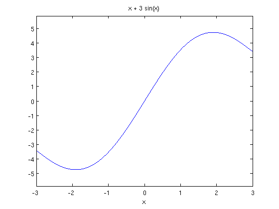
If you want to give it a specific domain of x values you can do that too:
ezplot(x+3*sin(x),-3,3)
Calculus 1
Take a derivative and then substitute:
subs(diff(x^3),x,3)
ans =

    27
Notice that subs is wrapped around diff. If we wrap diff around subs look at what happens and think about why:
diff(subs(x^3,x,3))
ans =

     []
Find an indefinite integral. Notice that Matlab, like many careless students, never puts a +C in its indefinite integrals. Grrr.
int(x*sin(x))
ans =

sin(x) - x*cos(x)
Find a definite integral.
int(x*sin(x),0,pi/6)
ans =

1/2 - (pi*3^(1/2))/12
Calculus 2
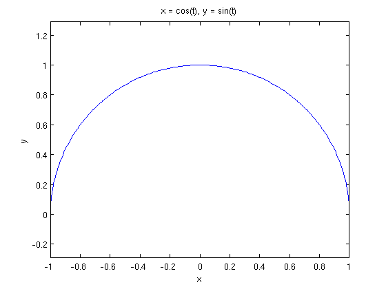
Plot the parametric curve x=cos(t), y=sin(t) for 0<=t<=pi. Note that this also a Calculus 3 problem if we think of this as plotting the VVF given by r(t) = cos(t) i + sin(t) j. Notice also the new symbolic variable t is declared.
syms t
ezplot(cos(t),sin(t),[0,pi])
Calculus 3
Define a vector. Vectors in Matlab are treated like in linear algebra so this may be new to you. The vector 2 i + 3 j + 7 k can be entered either as a horizontal vector or a vertical vector. Whatever you choose to use, be consistent. I will use horizontal vectors in this guide because that's how we think of them in Math 241. As a vertical vector we use semicolons to separate rows:
u=[2;3;7]
u =

     2
     3
     7
As a horizontal vector (like I'll do) we use spaces or commas. I'll use spaces out of habit.
u=[2 3 7]
u =

     2     3     7
We can put variables inside vectors too for VVFs and then take derivatives and stuff like that:
a=[t^2 1/t 2*t]
diff(a)
int(a,1,3)
a =

[ t^2, 1/t, 2*t]


ans =

[ 2*t, -1/t^2, 2]


ans =

[ 26/3, log(3), 8]
Here are various combinations of vectors. Notice also here the semicolons at the end of the first two lines. These semicolons suppress the output, meaning we're telling Matlab "assign the vectors and keep quiet about it". Also note the use of norm for the length (magnitude) of a vector. Don't use the Matlab command length because that just tells you how many elements are in the vector.
u=[6 9 12];
v=[-1 0 3];
norm(u)
w=u+v
dot(u,v)
cross(u,v)
dot(u,cross(u,v))
dot(u,v)/dot(v,v)*v
ans =

   16.1555


w =

     5     9    15


ans =

    30


ans =

    27   -30     9


ans =

     0


ans =

    -3     0     9
A few things to observe: The cross command produces a new vector, obviously. The second-to-last value is 0 and you should have expected that. Why? What is the last calculation finding? It's something familiar.
Here's the distance from the point (1,2,3) to the line with parametric equations x=2t, y=-3t+1, z=5. Make sure you see what's going on here. The point Q is off the line, the point P is on the line and the vector L points along the line. The reason P and Q are given as vectors is that we can then easily do Q-P to get the vector from P to Q.
Q=[1 2 -3];
P=[0 1 5];
L=[2 -3 0];
norm(cross(Q-P,L))/norm(L)
ans =

    8.1193
Warning: There are certain things which behave differently in Matlab than you might expect because Matlab knows a bit more than you might about some things. For example the dot product of two vectors has a more flexible definition if the entries are complex numbers. In the above example this was never an issue since neither u nor v is complex but if we try to use a variable look at what happens. Notice I've put clear all first which completely clears out Matlab so we know we're starting anew.
clear all;
syms t;
a=[t 2*t 5];
dot(a,a)
ans =

5*t*conj(t) + 25
What happened? Matlab doesn't know that t is a real number and so it does the more generic dot product which we are not familiar with. If we want Matlab to know that t is a real number we can tell it:
clear all;
syms t;
sym(t,'real');
a=[t 2*t 5];
dot(a,a)
ans =

5*t^2 + 25
That additional like sym(t,'real') tells Matlab to treat t as a real number so that conj stuff (complex conjugate) won't bother us.
Another Warning: Matlab's commands are sometimes annoyingly specific. For example the norm command only works on vectors with numerical entries. Doing norm([t 2*t 5]) will give an error. However we know that the norm of a vector is the square root of the dot product of the vector with itself. Thus:
a=[t 2*t 5];
sqrt(dot(a,a))
ans =

5^(1/2)*(t^2 + 5)^(1/2)
We might use this, for example, in finding the tangent and normal vectors for a VVF. Here we've done the curvature too just for fun.
r=[t t^2];
T=simplify(diff(r)/sqrt(dot(diff(r),diff(r))))
N=simplify(diff(T)/sqrt(dot(diff(T),diff(T))))
K=simplify(sqrt(dot(diff(T),diff(T)))/sqrt(dot(diff(r),diff(r))))
T =

[ 1/(4*t^2 + 1)^(1/2), (2*t)/(4*t^2 + 1)^(1/2)]


N =

[ -(2*t)/(4*t^2 + 1)^(1/2), 1/(4*t^2 + 1)^(1/2)]


K =

2/(4*t^2 + 1)^(3/2)
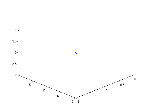
Okay, let's plot some stuff in three dimensions! Here is how we can plot just one point, the point (1,2,3):
plot3(1,2,3,'o')
view([10 10 10])
And here are two points:
plot3(1,2,3,'o',-1,2,5,'o')
view([10 10 10])
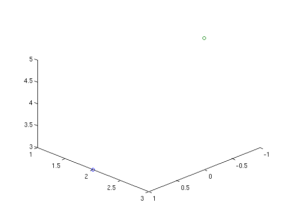
Note the 'o' tells Matlab to draw circles for points. Also note the view command there. Matlab has an annoying habit of viewing the axes from a nonstandard angle. The view([10 10 10]) command puts our point-of-view at the point (10,10,10) so we look down at the origin as we're used to in class.
Important observation! On the figure window there is a little rotation button which allows you to drag the picture around and look at it from different angles. Very useful and fun too! I can't demonstrate in a fixed html document though.
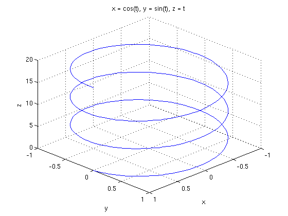
Okay now, let's plot some curves! We'll use the 3D command ezplot3. In class we sketched a helix with r(t)=cos(t)i+sin(t)j+tk.
ezplot3(cos(t),sin(t),t,[0,6*pi])
view([10 10 10])
Someone asked in class about what would happen if that third variable were also a trig function. Let's see. Also note that if we don't give it a t range it tries to find a nice one itself, just like ezplot did.
ezplot3(cos(t),sin(t),sin(t))
view([10 10 10])
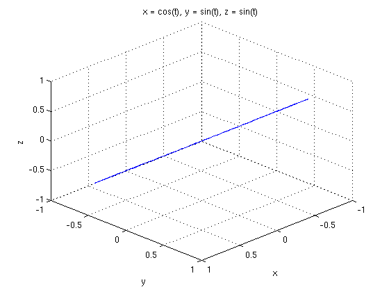
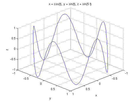
Okay that's a bit boring but it's happening because the frequency with which it oscillates up and down is the same as the frequency with which it rotates. Here's a better example in which the curve does one full rotation and while rotating it does five full up-down oscillations. We've also given it a specific range of t values. Try rotating that puppy for a really fun time!
ezplot3(cos(t),sin(t),sin(5*t),[0,2*pi])
view([10 10 10])
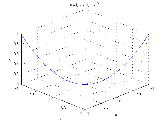
If you have a VVF defined already and wish to ezplot3 it then you need to give it the component functions. You can do this like:
r=[t -t t^2];
ezplot3(r(1),r(2),r(3),[-1,1])
view([10 10 10])
Here's a vector in 3D. The first three coordinates are the anchor point and the last three are the vector. So this is the vector 3i+4j-2k anchored at (1,2,3).
quiver3(1,2,3,3,4,-2)
view([10 10 10])
daspect([1 1 1])
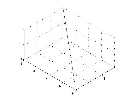
This last command daspect sets the aspect ratio so that all the axes are scaled the same. I have no idea why Matlab doesn't do this by default but grumble grumble grumble.
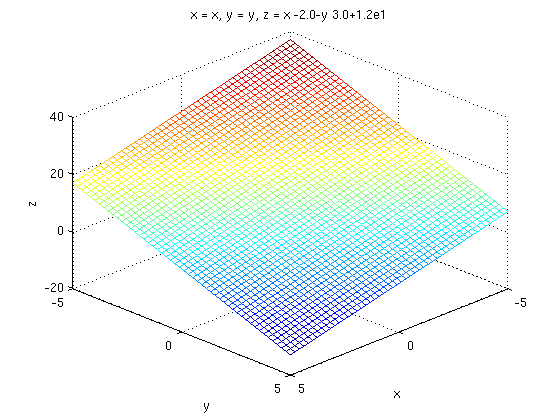
Just to close out let's draw some planes. These are not easy in Matlab in that we can't just throw the equation at it and expect good results. Instead here's the proces we need to take:
For example suppose we wish to plot 2*x+3*y+2*z=12. We solve for z=12-2*x-3*y and then we decide to use the suggested -5<=x<=5 and -5<=y<=5 and so we do:
syms x y z;
ezmesh(x,y,12-2*x-3*y,[-5,5,-5,5])
view([10 10 10])
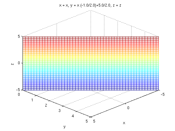
As another example suppose we wish to plot 2*x+4*y=10. We solve for y=(10-2*x)/4 and then we do the following. Notice that z is still there even though it's not part of the equation. In this case we have -5<=x<=5 and -5<=z<=5:
syms x y z;
ezmesh(x,(10-2*x)/4,z,[-5,5,-5,5])
view([10 10 10])
The end.