MATH/CMSC 206 - Introduction to Matlab

Answers to Self-Test

1. We would do something like this

fzero('x^2-5',2)

ans =

    2.2361

2. Simple!

fsolve('x^2-5',2)

Optimization terminated: first-order optimality is less than options.TolFun.

ans =

    2.2361

3. This works:

fsolve('x^3-25',2)

Optimization terminated: first-order optimality is less than options.TolFun.

ans =

    2.9240

4. Notice that this seems like it should work but then observe:

X=[-10:1:10];
plot(X,sec(X))

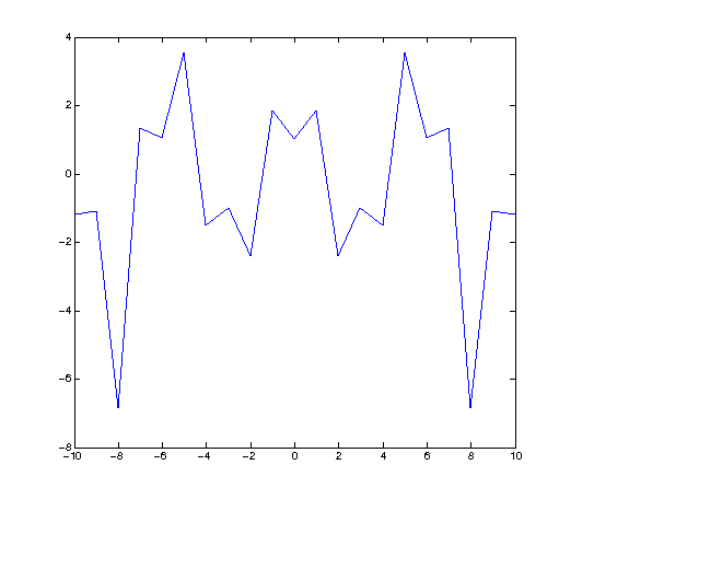
Wow! The problem you may see is obvious. We're using steps of 1 unit when we plot which means we've really got only 20 points plotted and consequently the result is jagged and unclear. This is a problem because we really don't see what the graph should look like.

5. It seems likely that in a fit of despair we figure we'll draw a really fine graph and so cut the steps down drastically:

X=[-10:0.001:10];
plot(X,sec(X))

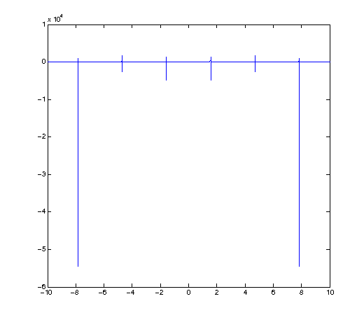
But from here we see another problem. What's happening is that the graph of secant has asymptotes and by picking such a small iteration we are guaranteed to get x-values near those asymptotes which result in very large positive and negative values. You can see this from the scale x10^4 at the corner of the graph. We're seeing such a vertically large region that all detail near y=0 is lost.

6. A good solution might be to pick a happy medium for the iteration and also to pick something somewhat related to trig functions in general - a multiple of pi.

X=[-10:pi/20:10];
plot(X,sec(X))

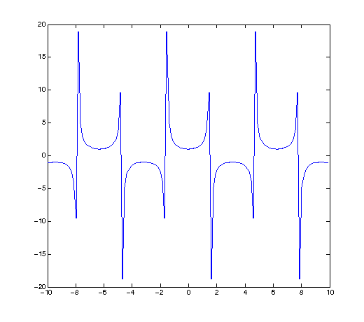
Ah, then we start to see the features!

7. Your first thought might be that the derivative has no roots. In general this could certainly be the case but it's not so here. In this case it's the fact that the derivative has a root but doesn't cross the x-axis at that root. Consequently fzero doesn't see it. If we try it with fsolve:

syms x;
f=@(x) x^5-6*x^4+16*x^3-32*x^2+48*x-32;
fsolve(inline(diff(f(x))),1)

Optimization terminated: first-order optimality is less than options.TolFun.

ans =

    1.9995

A quick jaunt into calculs would tell us that Matlab has found a close approximation to the root x=2.