MATH/CMSC 206 - Introduction to Matlab

Announcements

Syllabus

Tutorial

Projects

Submitting

More With Functions

Contents

More With Functions

Now that you know three of the four ways to define functions (symbolically, inline and with handles) let's briefly look at what each is really good for.

Differentiation of Functions

As differentation is a symbolic operation we must do it on the symblic definition of a function like this:

syms x;
f = 'x^3+2*x';
diff(f)

 
ans =
 
3*x^2 + 2
 

If you have an inline function or a function handle this might leave you wondering how to do the job. But Matlab is more flexible than you might think! Even though neither inline functions nor function handles are symbolic, their output is. In other words if f is an inline function or a function handle and x is symbolic then f(x) is symbolic. This means that the following will work just fine:

f = inline('x^3+exp(5*x)');
syms x;
diff(f(x))

 
ans =
 
5*exp(5*x) + 3*x^2
 

In a similar manner the following file handle example will work just fine:

g = @(x) x^2+x;
syms x;
diff(g(x))

 
ans =
 
2*x + 1
 

Of course since the result of diff is a symblic expression if we wish to plug something in we'll have to go back to the subs command. The following declares a function handle, differentiates the function and then plugs in a number:

g = @(x) x^2+x;
syms x;
subs(diff(g(x)),3)

ans =

     7

Integration of Functions

As was true for differentiation is true for integration. Consider the following which creates a file handle, converts it to a string and performs a definite integral:

g = @(x) sin(5*x)+tan(x)+x;
syms x;
int(g(x),0,pi/4)

 
ans =
 
log(2)/2 + 2^(1/2)/10 + pi^2/32 + 1/5
 

Numerical Integration

The commands quad and quadl will numerically integrate but only function handles and inline functions, not symbolic expressions. However we must recall that back when we learned the quad command we had to use our special operations .*, ./ and .^. So for example the following will work:

g = @(x) x.^2+sin(x);
quad(g,0,2)

ans =

    4.0828

The matlabFunction command

It often occurs that we have a symbolic expression and we wish to use quad on it. To do this we need to convert it to a function handle. Luckly the Matlab command matlabFunction does this. For example:

syms x
f=x^2+sin(x)
fh=matlabFunction(f)
quad(fh,0,pi)

 
f =
 
sin(x) + x^2
 

fh = 

    @(x)sin(x)+x.^2


ans =

   12.3354

Think about what this does. First x is defined symbolically, then f is defined symbolically in terms of x. Then the function handle fh is created. Lastly we apply quad. I've purposefully left of the semicolons so you can see the output of each step.

Now you might wonder why we didn't just define the function as a function handle to begin with and in this example you'd be right, it would be easier that way. But suppose you want to do the following: Suppose you want to define a function, take the derivative, square it and then apply quad. As you know the output from the derivative is symbolic so we have to somehow turn it back into a function handle before applying quad. Well, here we go:

f = @(x) x.^3+x;
syms x;
fh = matlabFunction(diff(f(x)));
quad(fh,-1,2)

ans =

    12

I've put the semicolons back in to keep it quiet but read through and think about what each step does. First define a function handle f. Define x symbolically so that f(x) is also symbolic. In the third line we apply diff(f(x)) which gives a symbolic answer which is then fed into matlabFunction to give a function handle result. This means that fh is a function handle and we can do quad in the final line.

Graphing

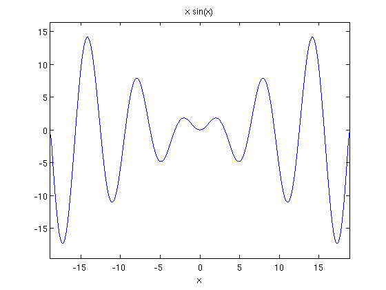
We saw earlier how ezplot can be used to graph functions as follows:

syms x;
ezplot(x*sin(x),[-6*pi,6*pi]);

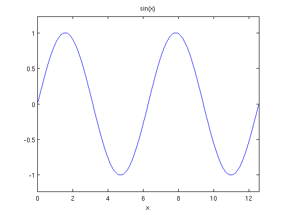
But what if you have a function defined in some manner and you wish to graph it? Can we use ezplot in these cases? Well the ezplot command is quite flexible and any of our three methods can be happily fed to it. That is, any of the following will work:

syms x;
f=sin(x);
ezplot(f,[0,4*pi])

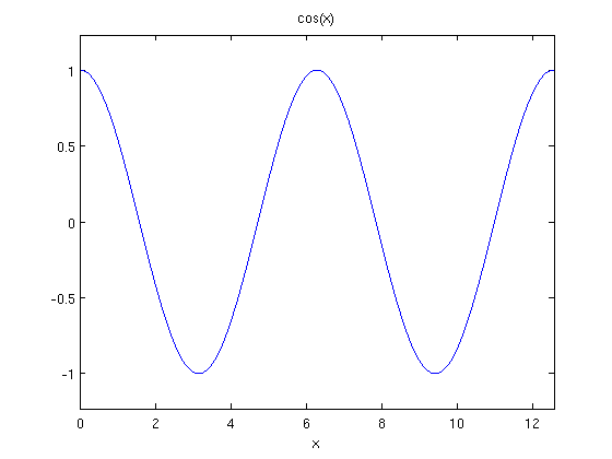
or

f=inline('cos(x)');
ezplot(f,[0,4*pi])

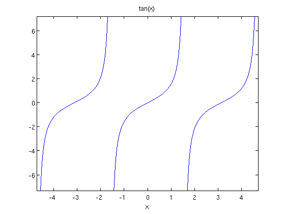
or

f=@(x) tan(x);
ezplot(f,[-3*pi/2,3*pi/2])

Finding Roots

Previously we saw the fzero command. This will work on either inline functions or function handles. It will not work on symbolic expressions though so to find a zero of a symbolic expression we would have to convert it first:

syms x;
f=x+exp(x);
fzero(inline(f),0)

ans =

   -0.5671

We can also use the solve command on function handles if we're careful. The trick is that f can be a function handle but f(x) (for symbolic x) is symbolic. Therefore for example:

f=@(x) x^2+2*x-6;
syms x;
solve(f(x))

 
ans =
 
 - 7^(1/2) - 1
   7^(1/2) - 1
 

Self-Test

Next Topic:   Programming with Matlab

Published with MATLAB® 7.9