Introduction to MATLAB®

copyright © 2011 by Jonathan Rosenberg, based on an earlier web page, copyright © 2000-2005 by Paul Green and Jonathan Rosenberg

Contents

Working with the Command Window

How MATLAB appears when it first launches depends to some extent on what kind of computer you are using and what defaults you have set, but in all cases you should see the MATLAB Desktop with a number of subwindows in it. The most important of these is the Command Window, where you should see a prompt symbol that looks like >>. Position your mouse there, type something, and hit Enter (or Return). This enables you to use MATLAB as a calculator. Here are some very simple examples:

1+1

sin(pi)

ans =

     2


ans =

  1.2246e-016

MATLAB has recognized sin as referring to the sine function, and pi as referring to . Of course , but because of round-off error, MATLAB has given the numerical answer (in scientific notation). That's because MATLAB does arithmetic with double-precision numbers, which are only accurate to around 15 decimal places. By default, MATLAB only prints five digits, but you can change this by typing format long and hitting RETURN. Thereafter, MATLAB will print out answers to 15 significant digits (unless you go back to the default by typing format short).

Exercise

Experiment with using the MATLAB Command Window as a calculator. The basic operations and functions are represented by * for "times", / for "divided by", ^ for powers (i.e., 3^3 means "3 cubed"), abs for absolute value, sqrt for square root, exp for the exponential function to the base e, so exp(1)=2.718281828..., log for the logarithm function to the base e, sin, cos, and tan for the basic trig functions, cosh, sinh, tanh for the basic hyperbolic functions, and asin, acos, atan for the inverse trig functions.

Numerical vs. Symbolic Calculation

It is important to remember that MATLAB, by default, does numerical calculations with double-precision numbers. It can also do exact, i.e., symbolic calculations and algebra, using an accessory called the Symbolic Math Toolbox, but only if you tell it to. For example, notice what happens if you type:

sin(sym('pi'))

 
ans =
 
0
 

The meaning of this is as follows. A string of characters, enclosed in single quotes, is what MATLAB calls a string. The command sym takes a string as an argument and tells MATLAB to interpret this string as a symbolic expression. So sym('pi') refers not to the approximate number 3.14159265... (which MATLAB denotes simply by pi) but to the exact symbolic number pi. So now when we take the sine, we get the exact answer 0. If you look carefully, you'll see that MATLAB indents its answer when the answer is numerical (double-precision) and prints its answer flush with the left margin when the answer is symbolic. That way you can always distinguish numerical from symbolic output.

The usual way to do symbolic calculations in MATLAB (to avoid having to keep writing such awkward expressions as sym('x') over and over) is to declare certain variables to be symbolic, usually with the syms command. Such a declaration lasts until you clear the assignment or assign a numerical value to that variable instead. Here's an example. Type

pi=sym('pi'); sin(pi)

 
ans =
 
0
 

and hit RETURN. That's equivalent to saying, "From now on I want pi to represent the true pi, not the approximation." The command syms declares whatever follows to be a symbolic variable or expression. Note that MATLAB responds without indentation. If you now type

clear pi

and hit RETURN, then type sin(pi) again and hit RETURN, you get back

sin(pi)

ans =

  1.2246e-016

Publishing M-files

The document you are currently reading may look like an ordinary web page, but it was produced by MATLAB as what is called a "published M-file". This is the recommended way to produce your homework assignments. From the MATLAB prompt in the Command Window, type edit followed by the name of a file (which must always end in .m --- MATLAB will insert this if you leave it out). This brings up an editor to create an "M-file". There are two kinds of M-files, function M-files and script M-files. For present purposes, you need a script M-files. The markup commands that produce section headings, etc., are produced with the Cell menu on the top Menu bar of the editor. Text should be put in a text cell (with lines starting with a percent sign), whereas MATLAB commands are in lines without a percent sign. When you are done writing your M-file, use the menu item on the File menu entitled Save file and publish ... to produce your web page. It may take several iterations to get everything the way you want it. Once you are done, you can print out your webpage and you have a document with embedded graphics, text, and MATLAB code.

Here's an example of a simple symbolic calculation with MATLAB.

syms x
factor(x^2-4)

 
ans =
 
(x - 2)*(x + 2)
 

Try creating such an input cell in your own M-file and evaluating it, either by running the M-file (by typing its name in the command window), or by using the Debug menu at the top of the editor, or by publishing the M-file.

Simple MATLAB Plots

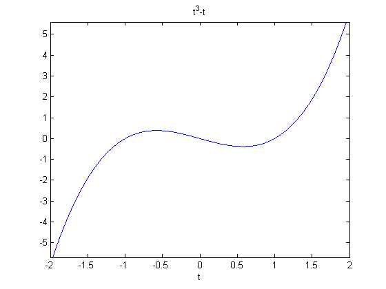
The easiest way to plot a graph in MATLAB is with the command ezplot. It can take as input either a string or a symbolic expression. Thus ezplot('t^3-t', [-2, 2]) and syms t followed by ezplot(t^3-t, [-2, 2]) are both acceptable ways to plot t^3 - t over the interval where t runs from -2 to 2. If you work in the Command Window, plots appear in separate figure windows. In a published M-file, they get incorporated into the final web page.

ezplot('t^3-t',[-2,2])

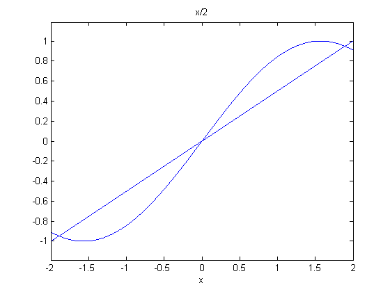
Once you have produced a plot, you can modify it. If the plot has been produced in a figure window, then commands to modify the plot will change the active figure window. If you are working in a publishable M-file with embedded figures, however, then commands to modify a plot must go in the same input cell as the plotting command. The command hold on sets a toggle switch so that output from the next plotting command s superimposed on the existing one. The command hold off turns this off again. Thus to find the solutions of the equation sin(x) = x/2, you can superimpose the plots of sin(x) and of x/2 as follows:

syms x; ezplot(sin(x),[-2,2]); hold on; ezplot(x/2,[-2,2]); hold off

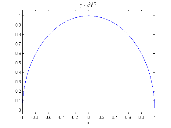
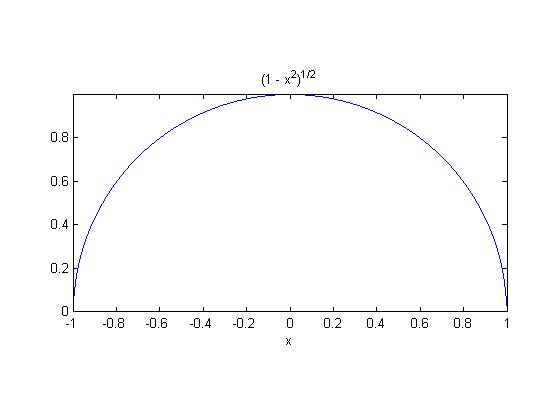
Note that you can separate commands on the same line with semicolons (or commas). A semicolon will also suppress the printed output (not the graphical output) of a command, but a comma will not. Another important command for modifying plots is the axis command, which enables you to modify the scales on the axes. For example, axis tight will cut the axes down to the minimum required to enclose the figure, and axis equal makes the scales on the horizontal and vertical axes the same. This is important to know about if you want your circles to look like circles and not like ellipses. Thus compare the following two ways to plot a semicircle:

ezplot(sqrt(1-x^2),[-1,1])

ezplot(sqrt(1-x^2),[-1,1]); axis equal; axis tight

Getting Help in MATLAB

To use MATLAB effectively, it's important to know how to look up the syntax for hundreds of commands that you can't possibly memorize. There are many ways to get online help. If you remember the name of a command, but can't remember its syntax or all its options, all you have to do is to look it up in the Function Browser or Product Help (you find these in the Help menu on the top menu bar). Alternatively, you can type help or doc followed by the name of the command. The command help prints out brief comments, while doc gets you the full documentation in the Product Help or Help Browser (in a separate help window). Here's an example:

help axis

 AXIS  Control axis scaling and appearance.
    AXIS([XMIN XMAX YMIN YMAX]) sets scaling for the x- and y-axes
       on the current plot.
    AXIS([XMIN XMAX YMIN YMAX ZMIN ZMAX]) sets the scaling for the
       x-, y- and z-axes on the current 3-D plot.
    AXIS([XMIN XMAX YMIN YMAX ZMIN ZMAX CMIN CMAX]) sets the
       scaling for the x-, y-, z-axes and color scaling limits on
       the current axis (see CAXIS). 
    V = AXIS returns a row vector containing the scaling for the
       current plot.  If the current view is 2-D, V has four
       components; if it is 3-D, V has six components.
 
    AXIS AUTO  returns the axis scaling to its default, automatic
       mode where, for each dimension, 'nice' limits are chosen based
       on the extents of all line, surface, patch, and image children.
    AXIS MANUAL  freezes the scaling at the current limits, so that if
       HOLD is turned on, subsequent plots will use the same limits.
    AXIS TIGHT  sets the axis limits to the range of the data.
    AXIS FILL  sets the axis limits and PlotBoxAspectRatio so that
       the axis fills the position rectangle.  This option only has
       an effect if PlotBoxAspectRatioMode or DataAspectRatioMode are
       manual.
 
    AXIS IJ  puts MATLAB into its "matrix" axes mode.  The coordinate
       system origin is at the upper left corner.  The i axis is
       vertical and is numbered from top to bottom.  The j axis is
       horizontal and is numbered from left to right.
    AXIS XY  puts MATLAB into its default "Cartesian" axes mode.  The
       coordinate system origin is at the lower left corner.  The x
       axis is horizontal and is numbered from left to right.  The y
       axis is vertical and is numbered from bottom to top.
 
    AXIS EQUAL  sets the aspect ratio so that equal tick mark
       increments on the x-,y- and z-axis are equal in size. This
       makes SPHERE(25) look like a sphere, instead of an ellipsoid.
    AXIS IMAGE  is the same as AXIS EQUAL except that the plot
       box fits tightly around the data.
    AXIS SQUARE  makes the current axis box square in size.
    AXIS NORMAL  restores the current axis box to full size and
        removes any restrictions on the scaling of the units.
        This undoes the effects of AXIS SQUARE and AXIS EQUAL.
    AXIS VIS3D  freezes aspect ratio properties to enable rotation of
        3-D objects and overrides stretch-to-fill.
 
    AXIS OFF  turns off all axis labeling, tick marks and background.
    AXIS ON  turns axis labeling, tick marks and background back on.
 
    AXIS(H,...) changes the axes handles listed in vector H.
 
    See also AXES, GRID, SUBPLOT, XLIM, YLIM, ZLIM.

    Overloaded methods:
       vrjoystick/axis

    Reference page in Help browser
       doc axis

Functions

Sometimes you will need to use a function, something that takes an input and produces an output. While we will learn later about other ways to create functions in MATLAB, the simplest method is to use the "at sign" @. Thus

f = @(x) x^2 - 3

f = 

    @(x)x^2-3

means "define f to be the function of x given by x^2 - 3". We can test this:

f(4)

ans =

    13

The answer is the same as 4^2 - 3 = 13.

The MATLAB Workspace

As you work in MATLAB, you will usually end up defining various variables and objects. These are saved in the MATLAB Workspace. There are two ways to inspect the contents of the Workspace: with the Workspace browser, usually found in the upper right-hand corner of the Desktop, or with the whos command. This lists all the currently defined variables and their "types" (double (i.e., double-precision numeric), string, symbolic, etc.). Most of the time you will see a variable called ans; MATLAB uses this for the last output that you did not explicitly store somewhere else, so the contents of ans will usually change many times during a session. Variables can be removed from the Workspace (for instance, to save memory space) with the clear command. Consider the following example.

a='pi'; b=sym('pi'); c=pi; whos

  Name      Size            Bytes  Class              Attributes

  a         1x2                 4  char                         
  ans       1x1                 8  double                       
  b         1x1               112  sym                          
  c         1x1                 8  double                       
  f         1x1                32  function_handle              
  x         1x1               112  sym                          

Here a is of type "char" (a string), b and x are of type "sym" (symbolic), and c is of type "double". f is of type "function_handle", which means the name for a function. Allowable variable names must be strings of letters, underscores, and numbers starting with a letter, but both upper-case and lower-case letters are allowed, and MATLAB distinguishes between them. Don't be fooled by the fact that the help lines for a command often refer to the command in all caps; MATLAB's built-in commands are almost always to be typed entirely in lower-case letters.

Problems for Practice

Published with MATLAB® 7.13