A Sample Non-Linear System: The Pendulum

Contents

The pendulum equation is x'' + c x' + k^2 sin x = 0, with k^2 = g/L. The constant c is a measure of the amount of friction or air resistance. We convert this to a system by setting y = x', so y' = x''. Then the equation becomes

If we multiply the equation by x', it becomes

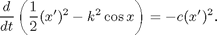
The quantity

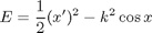
is called the energy.

The case of no friction

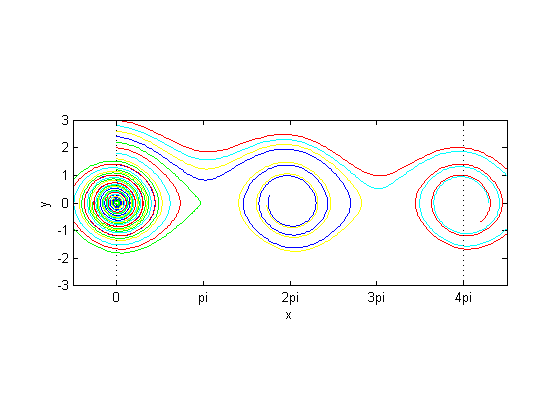
If there is no friction (i.e., c = 0), then dE/dt = 0, i.e., energy is conserved. Thus the trajectories lie along the level curves of E. Let's plot them for k = 1.

[xx, yy] = meshgrid((-.5:0.05:4.5)*pi, -3:0.05:3);
E = .5*yy.^2 - cos(xx);
contour(xx, yy, E)
axis equal
axis([0, 4*pi, -3, 3])
set(gca, 'XTick', (0:4)*pi)
set(gca, 'XTickLabel', {'0', 'pi', '2pi', '3pi', '4pi'})

The case of friction

Let's assume there is a small amount of friction, say c = 0.1. The critical points still lie at (n*pi, 0), n an integer. Let's compute the eigenvalues of the linearized system at (0, 0) and (pi, 0).

A1 = [0, 1; -1, -0.1]
eig(A1)

A1 =

         0    1.0000
   -1.0000   -0.1000


ans =

  -0.0500 + 0.9987i
  -0.0500 - 0.9987i

This is a stable spiral point.

A2 = [0, 1; 1, -0.1]
eig(A2)

A2 =

         0    1.0000
    1.0000   -0.1000


ans =

    0.9512
   -1.0512

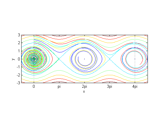
This is an unstable saddle point. Now let's plot some trajectories in the phase plane with ode45. The pictures show up best if we plot different trajectories in different colors.

colors = 'rgbyc';
rhs = @(t, x) [x(2); -0.1*x(2) - sin(x(1))];
options= odeset('RelTol', 1e-7);
for y0 = 0:15
    [t, x] = ode45(rhs, [0, 25], [0; 0.2*y0], options);
    plot(x(:,1), x(:, 2), colors(mod(y0,5)+1))
    hold on
end
plot([0,0],[-3,3],'k:',[4*pi,4*pi],[-3,3],'k:')
axis equal
axis([-pi/2, 4.5*pi, -3, 3])
xlabel 'x'
ylabel 'y'
set(gca, 'XTick', (0:4)*pi)
set(gca, 'XTickLabel', {'0', 'pi', '2pi', '3pi', '4pi'})

Energy plot

Now let's superimpose the contours of constant energy. Since the time derivative of energy is always non-positive, the trajectories most always be moving to states of lower energy.

contour(xx, yy, E)
hold off

Plots of x and y and functions of time

We can not only look at the phase plots but also at how x and y = dx/dt vary with time for the initial conditions we've chosen. Here are some pictures:

figure, hold on
for y0 = 0:0.2:3
    [t, x] = ode45(rhs, [0, 25], [0; y0], options);
    subplot(2, 1, 1), hold on
    plot(t, x(:,1))
    subplot(2, 1, 2), hold on
    plot(t, x(:, 2))
    hold on
end
subplot(2, 1, 1)
xlabel t
ylabel 'x = angle'
set(gca, 'YTick', (0:4)*pi)
set(gca, 'YTickLabel', {'0', 'pi', '2pi', '3pi', '4pi'})
subplot(2, 1, 2)
xlabel t
ylabel 'y = angular velocity'

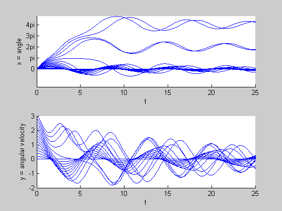
Note that the pictures confirm that as t goes to infinity, x tends to a multiple of 2pi and y tends to 0.

Published with MATLAB® 7.0