Examples of Homogeneous Linear Systems

Contents

Case of a Saddle Point

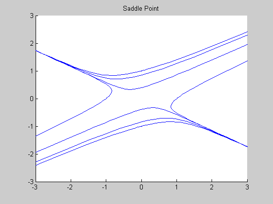
A = [1 3; 1 1]
eig(A)

A =

     1     3
     1     1


ans =

    2.7321
   -0.7321

Phase Portrait: let's take initial conditions spaced around a circle

figure, hold on
for j=1:8
    [t, y] = ode45(@(t, y) A*y, [0, 4], [cos(2*j*pi/8), sin(2*j*pi/8)]);
    plot(y(:,1), y(:, 2))
    [t, y] = ode45(@(t, y) A*y, [0, -4], [cos(2*j*pi/8), sin(2*j*pi/8)]);
    plot(y(:,1), y(:, 2))
end
axis([-3,3,-3,3]), hold off
title 'Saddle Point'

Case of a Spiral Point

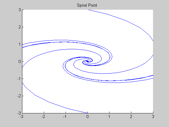
A = [1 -4; 1 1]
eig(A)

A =

     1    -4
     1     1


ans =

   1.0000 + 2.0000i
   1.0000 - 2.0000i

Phase Portrait: let's take initial conditions spaced around a circle

figure, hold on
for j=1:8
    [t, y] = ode45(@(t, y) A*y, [0, 4], [cos(2*j*pi/8), sin(2*j*pi/8)]);
    plot(y(:,1), y(:, 2))
    [t, y] = ode45(@(t, y) A*y, [0, -4], [cos(2*j*pi/8), sin(2*j*pi/8)]);
    plot(y(:,1), y(:, 2))
end
axis([-3,3,-3,3]), hold off
title 'Spiral Point'

Case of a Proper Node

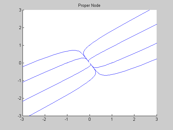
A = [2 1; 1 1]
eig(A)

A =

     2     1
     1     1


ans =

    2.6180
    0.3820

Phase Portrait: let's take initial conditions spaced around a circle

figure, hold on
for j=1:8
    [t, y] = ode45(@(t, y) A*y, [0, 4], [cos(2*j*pi/8), sin(2*j*pi/8)]);
    plot(y(:,1), y(:, 2))
    [t, y] = ode45(@(t, y) A*y, [0, -4], [cos(2*j*pi/8), sin(2*j*pi/8)]);
    plot(y(:,1), y(:, 2))
end
axis([-3,3,-3,3]), hold off
title 'Proper Node'

Published with MATLAB® 7.0