Now we want to look at the eigenpairs of
the stationary points to confirm our qualitative analysis. The stationary points
are the red and green points in the following plots.
| Stationary point 1 (5.6, -28.5, 28.5) |
Stationary point 2 (0.01, -0.035, 0.035) |
| Eigenvalue |
Eigenvector |
Eigenvalue |
Eigenvector |
| 0.1930 |
[0.01, -1, 1] |
0.0970 - i0.9952 |
[165 - i28, 11 + i167, 1.0] |
| i5.428 |
[0.0002 + i0.191, 0.035 - i0.001, 1] |
-5.687 |
[0.171, -0.029, 1.0] |
| -i5.428 |
[-i0.19, 0.04, 1] |
0.097 + i0.995 |
[164.8 + i28.3, 11.2 - i166.7, 1.0] |
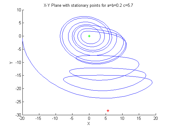
First we consider stationary point 1, which corresponds to the red, outlier point.
We have a pair of conjugate eigenvalues, with mu = 0, which indicates an ellipse, in
this case a counter-clockwise ellipse. We also have a positive real eigenpair,
indicating an unstable point, with the trajectories running away from this first stationary
point. For this point, we can see that these eigenpairs confirm the qualitative
analysis of the first stationary point, trajectories run away from the point towards
second stationary point, in an unstable elliptical fashion.
The second stationary point has a conjugate pair of eigenvalues with a positive mu,
which corresponds to a repelling spiral, which is contradictive to what we see in the plot.
But, this point also has a real eigenpair with a relatively large negative eigenvalue.
This last eigenpair indicates solutions run towards the point along the eigenvector.
These eigenpairs compete to create the chaotic action of the attractor around this
stationary point in the x,y-plane.
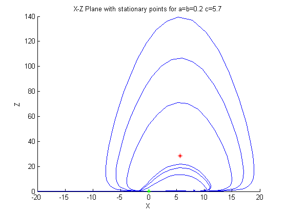
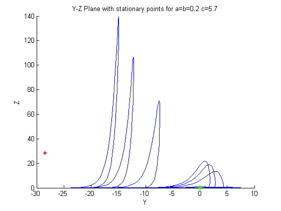
These two stationary points compete with each other, the first stationary point
helping to push trajectories spiraling towards the second, until they get caught in
the x,y-plane of the attractor, only to then be pulled again upwards and twisted in
the z-plane before falling back towards the x,y-plane. Below are the various phase
plane plots.
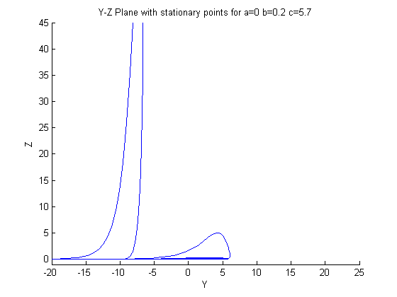
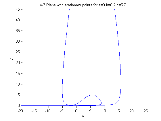
Second Case: a = 0
 This time we will lower the value of a, by a small amount
and observe how this affects the system. This system looks very similar to the above case,
but with one difference. There is no longer a strong pull from the outlier stationary point
and once the trajectory falls into the x,y-plane, it stays down in that plane and is not pulled
up in the z-axis. Again, we will look at the eigenvectors and hope to draw a qualitative conclusion.
This time we will lower the value of a, by a small amount
and observe how this affects the system. This system looks very similar to the above case,
but with one difference. There is no longer a strong pull from the outlier stationary point
and once the trajectory falls into the x,y-plane, it stays down in that plane and is not pulled
up in the z-axis. Again, we will look at the eigenvectors and hope to draw a qualitative conclusion.
| Stationary point 1 (5.7, -Inf, Inf) |
Stationary point 2 (0, NaN, NaN) |
| Eigenvalue |
Eigenvector |
Eigenvalue |
Eigenvector |
| undefined |
[0.01, -1, 1] |
undefined |
[165 - i28, 11 + i167, 1.0] |
| undefined |
[0.0002 + i0.191, 0.035 - i0.001, 1] |
undefined |
[0.171, -0.029, 1.0] |
| undefined |
[-i0.19, 0.04, 1] |
undefined |
[164.8 + i28.3, 11.2 - i166.7, 1.0] |
Regretfully, in this situation, we see that MATLAB cannot handle the calculations
necessary to determine the stationary points, and eigenvalues. We get a return of
either infinity or NaN (Not a Number), which is an undefined return. This helps to show
the very small range, in this case a change of only -0.1 to the coefficient a, needed to significantly
change the results. An interesting thing to note is the eigenvectors remained almost exactly the same as the first case.
Phase plots are shown below
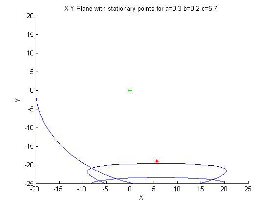
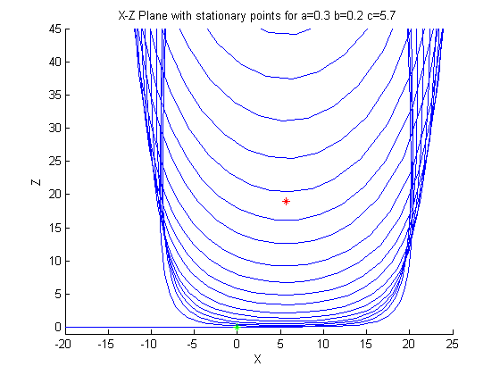
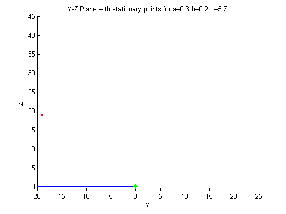
Third Case: a=0.3
 Now we will look at another very small
change in the coefficent a. This time changing it 0.1 greater than the first case. And again
we see the butterfly effect and witness a very large change in the system.
Now we will look at another very small
change in the coefficent a. This time changing it 0.1 greater than the first case. And again
we see the butterfly effect and witness a very large change in the system.
| Stationary point 1 (5.69, -18.96, 18.96) |
Stationary point 2 (0.011, -0.035, 0.035) |
| Eigenvalue |
Eigenvector |
Eigenvalue |
Eigenvector |
| 0.2845 |
[0.01, -1, 1] |
0.147 - i0.988 |
[165 - i28, 11 + i167, 1.0] |
| 0.0025 + i4.467 |
[0.0002 + i0.191, 0.035 - i0.001, 1] |
-5.6834 |
[0.171, -0.029, 1.0] |
| 0.0025 - i4.467 |
[-i0.19, 0.04, 1] |
0.147 + i0.988 |
[164.8 + i28.3, 11.2 - i166.7, 1.0] |
Two things that are immediately noticable about this system, all of the
eigenvectors are nearly exactly the same as the previous cases and there
has been a change in the first stationary points eigenvalues. The second stationary
point, the one close to the origin and corresponding to the chaotic spiral in the
x,y-plane has eigenvalues that can be considered the same as the first case, yet it's
attractive force is significantly smaller. We still have a positive real eigenpair,
indicating an unstable point, with the trajectories running away from this first stationary
point, as in the first case. But, this time, the conjugate pair of eigenvalues have a
positive mu, corresponding to a spiral source. What is most intersting about this
change is suddenly the attractor manifold is not trapping every solution so strongly into
the manifold. Instead we see the spiral source running from the first stationary point
in BOTH directions, causing the huge influence of this stationary point, that
can be seen in all the plots.
Conclusion
There are a few interesting conclusions we can draw from this short exploration
of the Rossler chaotic attractor. One of the most interesting is the significant changes
that are affected by such a small change in the parameters of the system. Over a range of only 0.3 we saw the system
transform from an attracting spiral, mostly constrained to the x,y-plane to a classic single
manifold attractor with an attracting spiral in the x,y-plane that has it's trajectories pulled
and twisted into the z-direction, to a system with a weakly attracting spiral that is
overwhelmed by it's "outlier" stationary point and looks like a spiral SOURCE in the
x,z-plane with barely a trace of the spiral sink in the x,y-plane.
MATLAB Code
Below is the MATLAB code that will produce the eigenmethods and graphs from
the first case. Hopefully someone will find this useful or interesting enough to further
explore this chaotic attractor.
Rossler eigenmethods and plots for case 1
clear all;
close all;
syms x y z t a b c;
A = [ 0 -1 -1 ; 1 a 0 ; z 0 x-c];
[V D] = eig(A);
xs = [ (c+sqrt(c^2-4*a*b))/2 (c-sqrt(c^2-4*a*b))/2 ];
ys = -[ (c+sqrt(c^2-4*a*b))/(2*a) (c-sqrt(c^2-4*a*b))/(2*a) ];
zs = [ (c+sqrt(c^2-4*a*b))/(2*a) (c-sqrt(c^2-4*a*b))/(2*a) ];
lam1 = [subs(D(1,1), {'x' 'y' 'z'}, {xs(1) ys(1) zs(1)}) subs(D(1,1), {'x' 'y' 'z'}, {xs(2) ys(2) zs(2)})];
lam2 = [subs(D(2,2), {'x' 'y' 'z'}, {xs(1) ys(1) zs(1)}) subs(D(2,2), {'x' 'y' 'z'}, {xs(2) ys(2) zs(2)})];
lam3 = [subs(D(3,3), {'x' 'y' 'z'}, {xs(1) ys(1) zs(1)}) subs(D(3,3), {'x' 'y' 'z'}, {xs(2) ys(2) zs(2)})];
lambda = [lam1 ; lam2 ; lam3];
eigv1 = [subs(V(:,1), {'x' 'y' 'z'}, {xs(1) ys(1) zs(1)}) subs(V(:,1), {'x' 'y' 'z'}, {xs(2) ys(2) zs(2)})];
eigv2 = [subs(V(:,2), {'x' 'y' 'z'}, {xs(1) ys(1) zs(1)}) subs(V(:,2), {'x' 'y' 'z'}, {xs(2) ys(2) zs(2)})];
eigv3 = [subs(V(:,3), {'x' 'y' 'z'}, {xs(1) ys(1) zs(1)}) subs(V(:,3), {'x' 'y' 'z'}, {xs(2) ys(2) zs(2)})];
lambda1 = subs(lambda, {a b c}, {0.2 0.2 5.7})
vector1 = subs(eigv1, {a b c}, {0.2 0.2 5.7})
vector2 = subs(eigv2, {a b c}, {0.2 0.2 5.7})
vector3 = subs(eigv3, {a b c}, {0.2 0.2 5.7})
xs1 = subs(xs, {a b c}, {0.2 0.2 5.7})
ys1 = subs(ys, {a b c}, {0.2 0.2 5.7})
zs1 = subs(zs, {a b c}, {0.2 0.2 5.7})
a = 0.2; b = 0.2; c = 5.7;
t = [0,50];
xinit = [-20 0 0];
ross = @(t, x) [-x(2)-x(3); x(1) + a*x(2); b + x(3)*(x(1) - c)];
[T, X] = ode45(ross, t, xinit);
figure; hold on;
plot3(X(:,1), X(:,2), X(:,3))
plot3(xs1(1), ys1(1), zs1(1), 'r*')
plot3(xs1(2), ys1(2), zs1(2), 'g*')
title('Rossler attractor with stationary points for a=b=0.2 c=5.7')
xlabel('X'); ylabel('Y'); zlabel('Z');
hold off;
figure('Color', [1 1 1]); hold on;
plot(X(:,1), X(:,2))
plot(xs1(1), ys1(1), 'r*')
plot(xs1(2), ys1(2), 'g*')
title('X-Y Plane with stationary points for a=b=0.2 c=5.7');
xlabel('X');
ylabel('Y');
hold off;
figure('Color', [1 1 1]); hold on;
plot(X(:,1), X(:,3))
plot(xs1(1), zs1(1), 'r*')
plot(xs1(2), zs1(2), 'g*')
title('X-Z Plane with stationary points for a=b=0.2 c=5.7');
xlabel('X');
ylabel('Z');
hold off;
figure('Color', [1 1 1]); hold on;
plot(X(:,2), X(:,3))
plot(ys1(1), zs1(1), 'r*')
plot(ys1(2), zs1(2), 'g*')
title('Y-Z Plane with stationary points for a=b=0.2 c=5.7');
xlabel('Y');
ylabel('Z');
hold off;
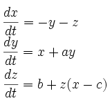 The Rossler attractor is a chaotic attractor that is a part of the Rössler
system. The attractor is defined by a non-linear system of three differential
equations, as seen on the right. This was designed by Otto Rossler in the
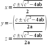
middle of the 20th century. This attractor has two stationary points, which can be found by the equations
on the left (found by solving the system for zero). For the purposes of this
demonstration, we will keep the coefficients b=0.2 and c=5.7 constant.
This will allow us to vary a, which will lead to significantly different
trajectory plots. By looking at the eigenpairs of the system near the stationary
points for different values of the coefficient a, we will be able to classify
the system qualitatively. In order to do all this, we'll need to employ some
eigenmethods to this system, but first we need to find the matrix A that represents this system.
This matrix is the Jacobian matrix of the system, seen below.
The Rossler attractor is a chaotic attractor that is a part of the Rössler
system. The attractor is defined by a non-linear system of three differential
equations, as seen on the right. This was designed by Otto Rossler in the
middle of the 20th century. This attractor has two stationary points, which can be found by the equations
on the left (found by solving the system for zero). For the purposes of this
demonstration, we will keep the coefficients b=0.2 and c=5.7 constant.
This will allow us to vary a, which will lead to significantly different
trajectory plots. By looking at the eigenpairs of the system near the stationary
points for different values of the coefficient a, we will be able to classify
the system qualitatively. In order to do all this, we'll need to employ some
eigenmethods to this system, but first we need to find the matrix A that represents this system.
This matrix is the Jacobian matrix of the system, seen below.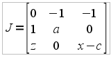
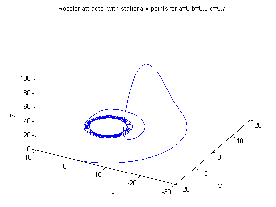
 This is a common set of coefficients
for studying the rossler function, and is rumored to be the original set of
coefficients studied by Rossler. With this set of coordinates, we can see
to the right that there are two competing stationary points, one in the center of
the manifold, an unstable spiral in the x,y plane and an outlying stationary
point that causes the trajectory to rise and twist along the z-axis before
falling back into the x,y plane.
This is a common set of coefficients
for studying the rossler function, and is rumored to be the original set of
coefficients studied by Rossler. With this set of coordinates, we can see
to the right that there are two competing stationary points, one in the center of
the manifold, an unstable spiral in the x,y plane and an outlying stationary
point that causes the trajectory to rise and twist along the z-axis before
falling back into the x,y plane.