Examples Wednesday, February 12
Contents
(a) Length of curve
Consider the curve r(t) = ( t, t^2, t^3 ) for t in [0,1.5] and find its length.
syms t real                        % declare t as real symbolic value
r = [t,t^2,t^3];
v = diff(r,t)                      % velocity
V = simplify(norm(v))              % speed
L = int(V,t,0,1.5)                 % integrate V for t=0 to 1.5
                                   % Matlab returns int(...) since it cannot find an antiderivative
L_numeric = vpa(L,7)               % use numerical integration to obtain 7-digit accuracy
v =
[ 1, 2*t, 3*t^2]
V =
(9*t^4 + 4*t^2 + 1)^(1/2)
L =
int((9*t^4 + 4*t^2 + 1)^(1/2), t == 0..3/2)
L_numeric =
4.597919
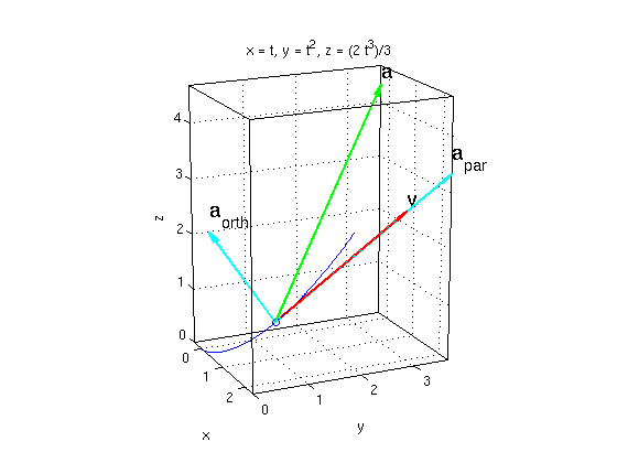
(b) Decomposition of the acceleration vector, change in speed V', curvature kappa
Consider the curve r(t) = ( t, t^2, (2/3)*t^3 ). Plot this curve for t in [0,1.5].
For t=1 plot the velocity vector v and the acceleration vector a.
Find the decomposition a = a_par + a_orth where a_par is parallel to v, a_orth is orthogonal on v. Use this to find the change of speed V' and the curvature kappa for this point.
r = [t,t^2,2/3*t^3];
v = diff(r,t)                      % velocity
a = diff(v,t)                      % acceleration
r0 = subs(r,t,1);                  % substitute t=1
v0 = subs(v,t,1)
a0 = subs(a,t,1)
V0 = norm(v0)                      % speed
a_par = dot(a0,v0)/dot(v0,v0)*v0   % acceleration component parallel to curve
a_orth = a0 - a_par                % acceleration component orthogonal to curve
kappa = norm(a_orth)/V0^2          % curvature
Vprime = dot(a0,v0)/V0             % change of speed

ezplot3(r(1),r(2),r(3),[0,1.5]); hold on
plotpts(r0,'o')
arrow3(r0,v0,'r'); texts(r0+v0,'v')
arrow3(r0,a0,'g'); texts(r0+a0,'a')
arrow3(r0,a_par,'c'); texts(r0+a_par,'a_{par}')
arrow3(r0,a_orth,'c'); texts(r0+a_orth,'a_{orth}')
hold off; nice3d
view(65,17)                        % pick nice angle to look at plot
v =
[ 1, 2*t, 2*t^2]
a =
[ 0, 2, 4*t]
v0 =
[ 1, 2, 2]
a0 =
[ 0, 2, 4]
V0 =
3
a_par =
[ 4/3, 8/3, 8/3]
a_orth =
[ -4/3, -2/3, 4/3]
kappa =
2/9
Vprime =
4
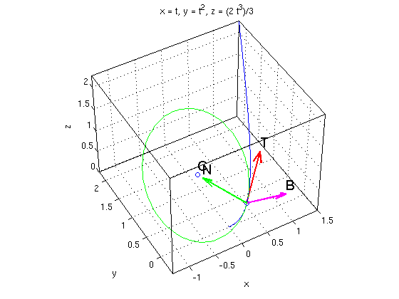
(c) Tangent vector T, normal vector N, binormal vector B, osculating circle
For the curve from (b) consider now the point with t=1/2. Find the unit tangent vector T, the normal vector N and the binormal vector B. Plot the curve with the vectors T, N,B and the osculating circle.
r0 = subs(r,t,1/2);                % substitute t=1/2 now
v0 = subs(v,t,1/2)
a0 = subs(a,t,1/2)
V0 = norm(v0)                      % speed
a_par = dot(a0,v0)/dot(v0,v0)*v0   % acceleration component parallel to curve
a_orth = a0 - a_par                % acceleration component orthogonal to curve
kappa = norm(a_orth)/V0^2          % curvature

T = v0/V0                          % unit tangent vector
N = a_orth/norm(a_orth)            % normal vector
B = cross(T,N)                     % binormal vector
R = 1/kappa                        % radius of osculating circle = 1/curvature
C = r0 + R*N                       % center of osculating circle

ezplot3(r(1),r(2),r(3),[0,1.5]); hold on
plotpts(r0,'o')
arrow3(r0,T,'r'); texts(r0+T,'T')
arrow3(r0,N,'g'); texts(r0+N,'N')
arrow3(r0,B,'m'); texts(r0+B,'B')
plotpts(C,'o'); texts(C,'C')
circle3(C,B,R,'g')                  % osculating circle
hold off; nice3d
view(-30,45)                        % pick nice angle to look at plot
v0 =
[ 1, 1, 1/2]
a0 =
[ 0, 2, 2]
V0 =
3/2
a_par =
[ 4/3, 4/3, 2/3]
a_orth =
[ -4/3, 2/3, 4/3]
kappa =
8/9
T =
[ 2/3, 2/3, 1/3]
N =
[ -2/3, 1/3, 2/3]
B =
[ 1/3, -2/3, 2/3]
R =
9/8
C =
[ -1/4, 5/8, 5/6]