Examples Monday, February 17
Contents
Curvature of Cycloid
Find the curvature of the cycloid as a function of t. Make a plot of this function for t in [0,2*pi].
syms t real
Pi = sym('pi');
r = [t-sin(t), 1-cos(t), 0];
v = diff(r,t)
a = diff(v,t)

kappa = simplify( norm(cross(a,v))/norm(v)^3 ) % formula with cross product
ezplot(kappa,[0,2*pi])                         % Plot kappa
title('curvature \kappa(t)')                   % Note: kappa becomes infinite for t=0, 2*pi
v =
[ 1 - cos(t), sin(t), 0]
a =
[ sin(t), cos(t), 0]
kappa =
2^(1/2)/(4*(1 - cos(t))^(1/2))

Vectors T, N and osculating circle
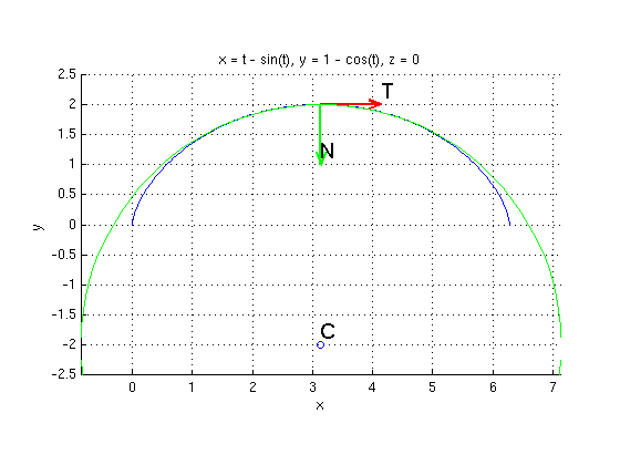
For t=pi find kappa, T, N. Plot the cycloid together with the osculating circle at t=pi.
(Try also other values like pi/2.)
t0 = Pi;                                       % Try also t0 = Pi/2
r0 = subs(r,t,t0);                             % Plug in t=t0
v0 = subs(v,t,t0);
a0 = subs(a,t,t0);
apar = dot(a0,v0)/dot(v0,v0)*v0;               % decompose a0 = apar + aorth
aorth = simplify(a0 - apar);
kappa0 = subs(kappa,t,t0);                     % curvature, same as norm(aorth)/dot(v0,v0)
T = v0/norm(v0)                                % unit tangent vector T
N = aorth/norm(aorth)                          % normal vector N
B = cross(T,N);                                % binormal vector
R = 1/kappa0                                   % radius of osculating circle
C = r0 + R*N                                   % center of osculating circle

ezplot3(r(1),r(2),r(3),[0,2*pi]); hold on      % plot curve for t=0...2*pi
arrow3(r0,T,'r'); texts(r0+T,'T')
arrow3(r0,N,'g'); texts(r0+N,'N')
plotpts(C,'o'); texts(C,'C')
circle3(C,B,R,'g')                             % plot osculating circle (green)
hold off; axis equal
ylim([-2.5 2.5])                               % show y between -2.5, 2.5
view(0,90);                                    % look at xy-plane
T =
[ 1, 0, 0]
N =
[ 0, -1, 0]
R =
4
C =
[ pi, -2, 0]