- Problem 1
-
Typos: Use [-2,2] as the range for both
y1 and y2. Find the behavior as
t (not y ) goes to infinity.
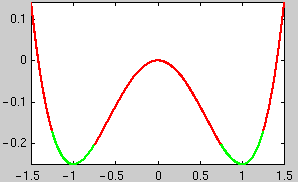 Mechanical interpretation of
ODE: y(t) describes the horizontal position of a
ball rolling in a curve with two valleys. In the red areas energy is taken out
of the ball by positive damping, and in the green areas energy is pumped into
the ball by ``negative damping''.
Mechanical interpretation of
ODE: y(t) describes the horizontal position of a
ball rolling in a curve with two valleys. In the red areas energy is taken out
of the ball by positive damping, and in the green areas energy is pumped into
the ball by ``negative damping''.
Hints: Plot the vector field and trajectories as explained on
the page for autonomous problems. Use
larger ranges for t such as [0,20] and
[0,-20] (instead of [0,4] and [0,-4]).
First plot only one trajectory and investigate what happens for large values
of t.
To find the critical points symbolically proceed as on the page for autonomous problems. But because of
a design flaw in Matlab, instead of
[y1s,y2s]=solve(G(1),G(2),y1,y2) you must use
[y1s,y2s]=solve(2*G(1),G(2),y1,y2) (otherwise Matlab confuses
equations and variables).
- Problem 2(a)
-
Typo: Use [0,12] for the t-range (not [0,7]).
The easiest way to define the function g is to use an m-file
called g.m which looks like this:
function yprime=g(t,y)
a = 1/82.45; b = 1-a;
r1 = sqrt( ... );
r2 = sqrt( ... );
yprime = [ ... ;
           ... ;
           ... ;
           ... ];
Note that you then have to use ode45('g',...) (with quotes around
g) to use the function defined in an m-file.
The trajectory should be plotted in the (x, y)- plane (i.e.,
the (y1,y2)-plane). The page about higher order ODEs and systems
explains two methods for plotting trajectories. Both methods work here.
- Problem 2(b)
-
Typo: The point should be (0.3, 0), not
(1.3, 0). Make plots of the trajectories in the (x,y) plane
as explained above.
- Problem 2(c)
We want to put the satellite at a spot where it stays at a fixed position with
respect to the rotating earth-moon system. This corresponds to a critical
point of our system.
(Actually, Al Gore wants to put the satellite at a fixed point in the rotating
sun-earth system, not the rotating earth-moon system. This would have the
advantage that the satellite could always see the day side of the earth. But
the satellite would be much further away, and it would be at an unstable
critical point. Here is more
information about Al Gore's idea.)
To find the critical points symbolically proceed as on the web page for autonomous problems. But
because of a design flaw in Matlab, instead of
[y1s,y2s,y3s,y4s]=solve(G(1),G(2),G(3),G(4),y1,y2,y3,y4) you
must use
[y1s,y2s,y3s,y4s]=solve(2*G(1),2*G(2),G(3),G(4),y1,y2,y3,y4)
(otherwise Matlab confuses equations and variables). Note that we are only
interested in real solutions.
To find the critical points numerically: Either use
fsolve (available on Glue, WAM, but not in the student version of
Matlab). Make an m-file called g1.m which is identical to
g.m, except for the first line function
yprime=g1(y). Then use fzero('g1',guess) where
guess is of the form [c1;c2;0;0] containing an
initial guess for the critical point.
Or: just try to find the three solutions with y2=0. This reduces
the problem to finding zeros of one function of one variable, which you can do
using the command fzero.
To find the eigenvalues of the Jacobian: If you have problems
with a command like eig(jac1) try using
eig(double(jac1)). If jac1 is a symbolic matrix,
eig(jac1) tries to find eigenvalues symbolically, and
eig(double(jac1)) tries to find eigenvalues numerically.