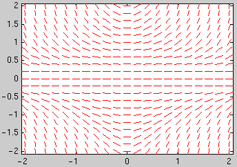
dirfield(g,-2:0.2:2,-2:0.2:2)

If you want to use a function several times it is convenient to define it as a so-called inline function:
f1 = inline('sin(x).*x','x')
defines the function f1(x)=sin(x).*x. Note that the arguments of
inline must be strings (not symbolic expressions). You
can then use the function f1 in expressions you type in.
You must always use ``.*'',
``./'', ``.^'' instead of ``*'',
``/'', ``^'' in your functions. In this way you can
apply the function to a whole vector of values at the same time. E.g., you can
plot your function using
t = -10:.1:10; plot(t,f1(t))
You can also define inline functions of several variables:
g1 = inline('x.*y+sin(x)','x','y')
defines the function g1(x,y)=x.*y+sin(x) of two variables.
First save the file dirfield.m into your home
directory.
Define an inline function g of
two variables t, y corresponding to the right hand
side of the differential equation y'(t) =
g(t,y(t)). E.g., for the differential
equation y'(t) = t y2
define
g = inline('t.*y.^2','t','y')
Remember to always use ``.*'', ``./'',
``.^''. You have to use inline(...,'t','y'), even if
t or y does not occur in your formula.
To plot the direction field for t going from t0 to t1 with a
spacing of dt and y going from y0 to y1 with a spacing of dy use
dirfield(g,t0:dt:t1,y0:dy:y1). E.g., for
t and y between -2 and 2 with a spacing of 0.2
type
dirfield(g,-2:0.2:2,-2:0.2:2)
First define the inline function
g corresponding to the
right hand side of the differential equation y'(t) =
g(t,y(t)). E.g., for the differential
equation y'(t) = t y2
define
g = inline('t.*y.^2','t','y')
To plot the numerical solution of an initial value
problem: For the initial condition y(t0)=y0 you can plot the
solution for t going from t0 to t1 using
ode45(g,[t0,t1],y0).
Example: To plot the solution of the initial value problem y'(t) = t y2, y(-2)=1 in the interval [-2,2] use
ode45(g,[-2,2],1)
The circles mark the values which were actually computed (the points are
chosen by Matlab to optimize accuracy and efficiency). You can obtain vectors
ts and ys with the coordinates of these points using
[ts,ys] = ode45(g,[t0,t1],y0). You can then plot
the solution using plot(ts,ys) (this is a way to
obtain a plot without the circles).
To combine plots of the direction field and several
solution curves use the commands hold
on and hold off: After obtaining
the first plot type hold on, then all subsequent commands plot in
the same window. After the last plot command type hold off.
Example: Plot the direction field and the 13 solution curves with the initial conditions y(-2) = -0.4, -0.2, ..., 1.8, 2:
dirfield(g,-2:0.2:2,-2:0.2:2)
hold on
for y0=-0.4:0.2:2
  [ts,ys] = ode45(g,[-2,2],y0); plot(ts,ys)
end
hold off
To obtain numerical values of the solution at certain t
values: You can specify a vector tv of t values and
use [ts,ys] = ode45(g,tv,y0). The first element
of the vector tv is the initial t value; the vector
tv must have at least 3 elements. E.g., to obtain the solution
with the initial condition y(-2)=1 at t = -2, -1.5, ..., 1.5, 2 and
display the results as a table with two columns, use
[ts,ys]=ode45(g,-2:0.5:2,1);

[ts,ys]