Compute discrete convolution, deconvolution using discrete Fourier transform
Contents
Given signal and filter
four = @(f) fft(f)/length(f);    % discrete Fourier transform as defined in class
ifour = @(f) ifft(f)*length(f);

N = 128;
t = (0:N-1)/N;
u = 0:N-1;                         % signal

M = 30;                            % filter has coefficients from -M,...,M
v = [M:-1:0,zeros(1,N-2*M),1:M-1]; % filter
v = v/sum(v)*N;                    % normalize so that filter gives weighted averages

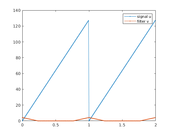
plot([t,t+1],[u,u],'.-'); hold on
plot([t,t+1],[v,v],'.-');
legend('signal u','filter v')
Find discrete Fourier transforms
uh = four(u);
vh = four(v);
wh = uh.*vh;                       % convolution in frequency domain
w = ifour(wh);

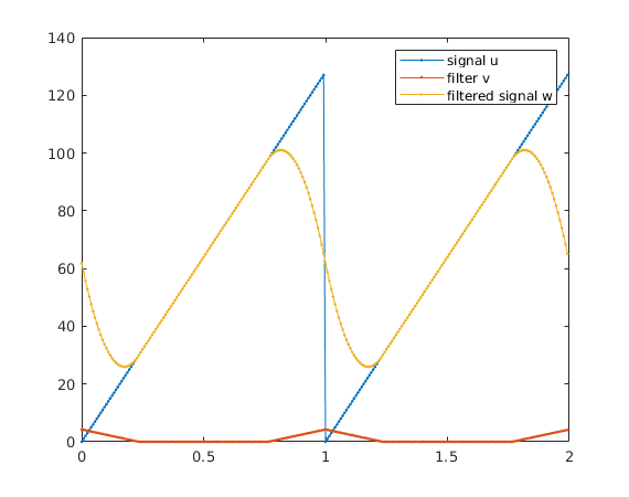
plot([t,t+1],[w,w],'.-')
legend('signal u','filter v','filtered signal w')
hold off
Given exact w, v: perform deconvolution to find u
wh = four(w);
vh = four(v);
Uh = wh./vh;                       % deconvolution in frequency domain
U = ifour(Uh);                     % reconstructed signal u

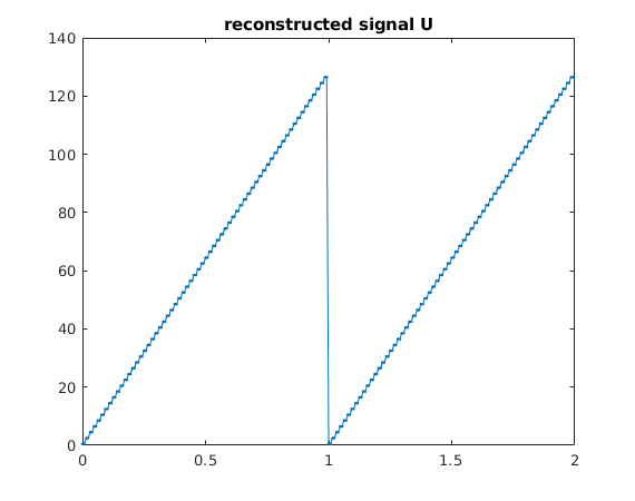
plot([t,t+1],[U,U],'.-')
title('reconstructed signal U')
snapnow

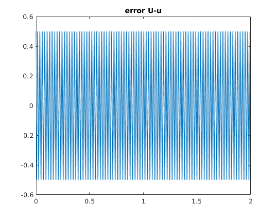
e = U-u;                           % error
plot([t,t+1],[e,e])
title('error U-u')
Given noisy version W of w: try to perform naive deconvolution
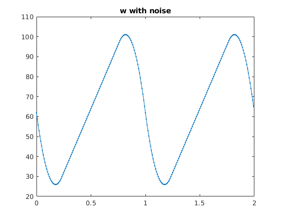
We add a tiny amount of noise.
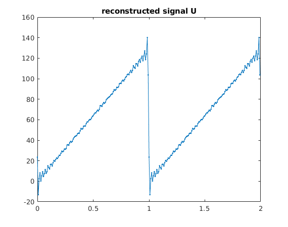
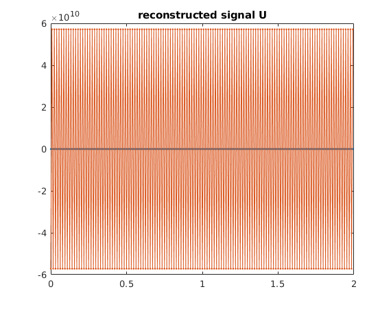
Now the deconvolution hugely magnifies this noise and completely dominates over the reconstructed signal.
W = w + 1e-4*randn(1,N);           % add noise of size 1e-4
plot([t,t+1],[W,W],'.-')
title('w with noise')
hold on
snapnow

Wh = four(W);
vh = four(v);
Uh = Wh./vh;                       % deconvolution in frequency domain
U = ifour(Uh);                     % reconstructed signal u

plot([t,t+1],[U,U],'.-')
title('reconstructed signal U'); hold off
Given noisy version W of w: try to perform deconvolution, omitting very high frequencies
The trouble comes from the high frequencies.
Therefore we use zero for frequencies higher than K. Recall that frequencies higher than  correspond to
  .
.
K = 40;
Uh = Wh./vh;                       % deconvolution in frequency domain
Uh(K+2:end-K) = 0;                 % set all frequencies>K to zero
U = ifour(Uh);                     % reconstructed signal u

plot([t,t+1],[U,U],'.-')
title('reconstructed signal U')
