Solving a nonlinear least squares problem with the Gauss-Newton method and lsqnonlin
Contents
You need to download an m-file
Download the following m-file and put it in the same directory with your other m-files:
Given: three functions f1, f2, f3 of two variables x1,x2
Consider the functions

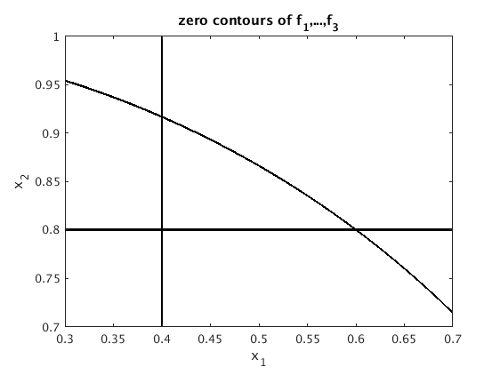
Below are the zero contours of the three functions. We see that there is no point where all three functions are zero.
f = @(x) [ x(1)-.4; x(2)-.8 ; x(1)^2+x(2)^2-1 ];

zerocont2m(f,[.3 .7 .7 1]) % plot zero contours of the functions f_1, f_2, f_3
hold on

Least squares problem: minimize norm(f)
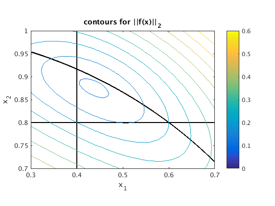
As we cannot achieve f(x)=[0;0;0] we want to find x such that norm(f(x)) is minimal. Below is a contour graph for norm(f(x)). We see that there is a point x where norm(f(x)) is minimal.
g = @(x1,x2) norm(f(x1*[1;0]+x2*[0;1]));  % we want to plot contour levels of g
ezcontour(g,[.3 .7 .7 1]); colorbar       % make contour plot (ignore warning)
title('contours for ||f(x)||_2')
Warning: Function failed to evaluate on array inputs; vectorizing the function
may speed up its evaluation and avoid the need to loop over array elements.

Gauss-Newton method
We first define the function fp(x) for the Jacobian matrix.
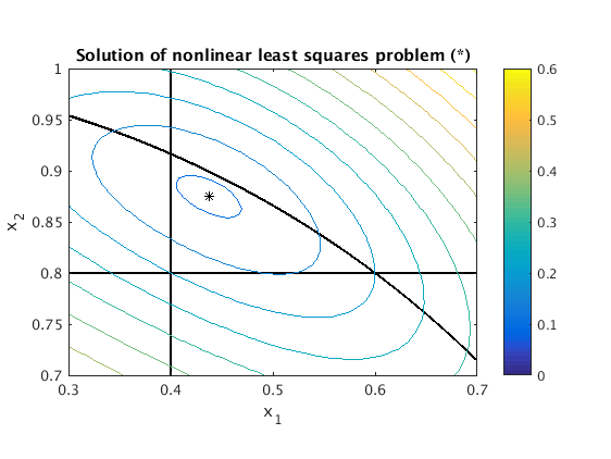
We start with the initial guess x=[0;0]. We see that the iteration converges to the point x = [.43752,.87504]. At this point norm(f(x)) has the minimal value .0942208.
fp = @(x) [ 1,0 ; 0,1 ; 2*x(1),2*x(2) ];  % define Jacobian fp(x)

format long g        % show all digits
x = [0;0];           % initial guess
while 1
  b = f(x);          % evaluate f
  A = fp(x);         % evaluate Jacobian
  d = -A\b;          % solve linear least squares problem norm(A*d+b)=min
  x = x + d
  if norm(d)<=1e-15  % stop iteration if norm(d)<=StepTolerance
    break
  end
end

fnorm = norm(f(x))   % norm of f(x) at minimum

plot(x(1),x(2),'k*'); hold off %    mark solution point with '*'
title('Solution of nonlinear least squares problem (*)')
x =
                       0.4
                       0.8
x =
         0.438095238095238
         0.876190476190476
x =
         0.437531075791456
         0.875062151582913
x =
         0.437520778200845
         0.875041556401689
x =
         0.437520595215861
         0.875041190431722
x =
         0.437520591965889
         0.875041183931778
x =
         0.437520591908167
         0.875041183816335
x =
         0.437520591907142
         0.875041183814284
x =
         0.437520591907124
         0.875041183814248
x =
         0.437520591907124
         0.875041183814247
fnorm =
        0.0942207695878639

Find errors for Gauss-Newton method
We have found a solution. We now run the iteration again to print the errors.
We see that the error improves by a factor of about .0178 with each iteration. Therefore we have convergence of order 1.
xs = x;              % xs is exact solution which we just found
x = [0;0];
enormold = NaN;
for i=1:10
  b = f(x);
  A = fp(x);
  d = -A\b;
  x = x + d;
  enorm = norm(x-xs);
  fprintf('enorm = %g, quotient = %g\n',enorm,enorm/enormold)
  enormold = enorm;
end
enorm = 0.0838986, quotient = NaN
enorm = 0.00128495, quotient = 0.0153155
enorm = 2.34427e-05, quotient = 0.0182441
enorm = 4.16565e-07, quotient = 0.0177695
enorm = 7.39856e-09, quotient = 0.0177609
enorm = 1.31404e-10, quotient = 0.0177607
enorm = 2.33383e-12, quotient = 0.0177608
enorm = 4.14583e-14, quotient = 0.0177641
enorm = 7.4476e-16, quotient = 0.0179641
enorm = 0, quotient = 0
Solving the nonlinear least squares problem with lsqnonlin
You can solve a nonlinear least squares problem |f(x)|=min using lsqnonlin. This has the following advantages:
- You only need to specify the function f, no Jacobian needed
- It works better than Gauss-Newton if you are too far away from the solution
- There are many options available: you can specify StepTolerance, FunctionTolerance, you can use the Jacobian, display information after each iteration etc. Type doc lsqnonlin for more details.
f = @(x) [ x(1)-.4; x(2)-.8 ; x(1)^2+x(2)^2-1 ];  % define f
x0 = [0;0];                                       % initial guess
[xs,fnorm2] = lsqnonlin(f,x0)                     % find solution xs
fnorm = sqrt(fnorm2)
Local minimum possible.

lsqnonlin stopped because the final change in the sum of squares relative to
its initial value is less than the default value of the function tolerance.


xs =
         0.437520778647501
         0.875041556336608
fnorm2 =
       0.00887755342255288
fnorm =
        0.0942207695922342