Contents

Optimization: Function of several variables

function optim2

You need to download an m-file

Download the following m-file and put it in the same directory with your other m-files:

Example function

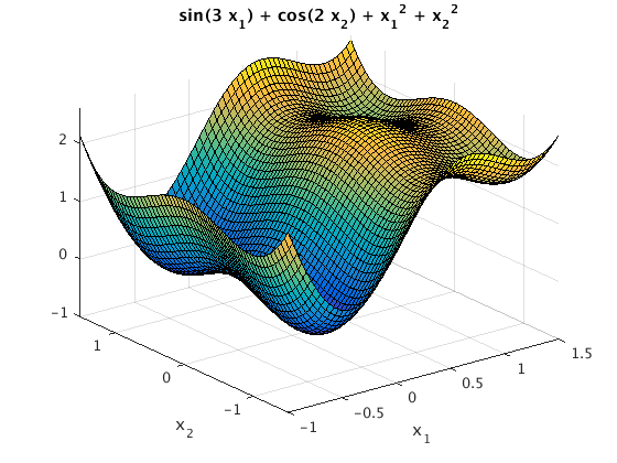
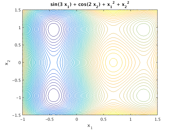
We want to find a local minimum of f(x) = sin(3*x1) + cos(2*x2) + x1^2 + x2^2

In the plots below we can see 4 local minima, 1 local maximum and 4 saddle points.

We can use a separate m-file f.m to define the function. Here we define the function as an "inner function" in the same m-file (see below).

figure(1)                      % make a surface plot
ezsurf('sin(3*x1) + cos(2*x2) + x1^2 + x2^2', [-1 1.5 -1.5 1.5])

figure(2)                      % make a contour plot
ezcontourc('sin(3*x1) + cos(2*x2) + x1^2 + x2^2', [-1 1.5 -1.5 1.5],50)
hold on

Using fminunc without the gradient

We use the function y=f(x) given below which only returns y, not the gradient.

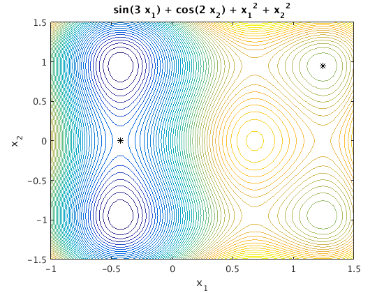
First we start at [0,0]. Matlab finds the point xs = [-.4273,0]. At this point the gradient is zero, but this is not a local minimum. It is actually a saddle point.

Then we start at [0,0]. Matlab finds the point xs = [1.2446,.9477]. This point is really a local minimum.

xs = fminunc(@f,[0,0])          % start at [0,0]
plot(xs(1),xs(2),'k*')

xs = fminunc(@f,[1,1])          % start at [1,1]
plot(xs(1),xs(2),'k*'); hold off

Warning: Gradient must be provided for trust-region algorithm; using
quasi-newton algorithm instead. 

Local minimum found.

Optimization completed because the size of the gradient is less than
the default value of the function tolerance.



xs =
   -0.4273    0.0000
Warning: Gradient must be provided for trust-region algorithm; using
quasi-newton algorithm instead. 

Local minimum found.

Optimization completed because the size of the gradient is less than
the default value of the function tolerance.



xs =
    1.2446    0.9477

Using fminunc with the gradient

We use the function [y,g]=F(x) given below which returns y and the gradient g.

First we start at [0,0]. Matlab finds the point xs = [-.4273,0]. At this point the gradient is zero, but this is not a local minimum. It is actually a saddle point.

Then we start at [0,0]. Matlab finds the point xs = [1.2446,.9477]. This point is really a local minimum.

Note that we found the same points as before, but this time fewer function evaluations were needed since the gradient was available (you can see this by using [xs,fval,exitflag,output] = fminunc(...) )

opt = optimset('GradObj','on'); % This is how to specify options for fminunc
xs = fminunc(@F,[0,0],opt)      % start at [0,0]
xs = fminunc(@F,[1,1],opt)      % start at [1,1]

Local minimum found.

Optimization completed because the size of the gradient is less than
the default value of the function tolerance.



xs =
   -0.4273         0

Local minimum found.

Optimization completed because the size of the gradient is less than
the default value of the function tolerance.



xs =
    1.2446    0.9477

Definition of f, F

The function f only returns the function value.

The function F returns also the gradient g if we use [y,g]=F(x)

function y = f(x)
y = sin(3*x(1)) + cos(2*x(2)) + x(1).^2 + x(2).^2;
end

function [y,g] = F(x)
y = sin(3*x(1)) + cos(2*x(2)) + x(1).^2 + x(2).^2;
g = [3*cos(3*x(1))+2*x(1); -2*sin(2*x(2))+2*x(2)];

end

end

Published with MATLAB® R2015a