Assignment #1, Problem 4
Contents
Solving linear system (i)
Gaussian elimination gives a matrix U with nonzero diagonal elements, hence there is a unique solution.
A = [1,2;2,1]
[L,U,p] = lu(A,'vector'); U            % matrix U from Gaussian elimination
b = [3;4]
x = A\b                                % unique solution
A =
     1     2
     2     1
U =
            2            1
            0          1.5
b =
     3
     4
x =
       1.6667
      0.66667
Plotting lines for linear system (ii)
The two lines intersect in a single point x which is the solution of the linear system we found before.
L1 = diag( b(1)./A(1,:) )              % two points satisfying eq.1
L2 = diag( b(2)./A(2,:) )              % two points satisfying eq.2

plotpoints(L1); hold on                % plot line for eq.1
plotpoints(L2,'--')                    % plot line for eq.2
plotpoints(x,'ko'); label(x,'x')       % plot solution point
hold off
axis equal; grid on; title('Two lines intersect at solution point x')
legend('equation 1','equation 2')
L1 =
            3            0
            0          1.5
L2 =
     2     0
     0     4

Solving linear system (ii)
Gaussian elimination fails, it does not give matrix U with nonzero diagonal elements. Hence the matrix A is singular. So the linear system has either no solution or infinitely many solutions.
Using \ with machine arithmetic gives a warning that the matrix is singular within machine precision.
Using \ with symbolic arrays gives a message that no solution exists.
A = [1,2;2,4]
[L,U,p] = lu(A,'vector'); U            % matrix U from Gaussian elimination
b = [3;4]
% Using Matlab with machine arithmetic
x = A\b                                % Matlab gives Inf (infinity)
% Using symbolic computation:
x = sym(A)\sym(b)                      % symbolic \ gives warning that no solution exists
A =
     1     2
     2     4
U =
     2     4
     0     0
b =
     3
     4
Warning: Matrix is singular to working precision.
x =
   Inf
  -Inf
Warning: The system is inconsistent. Solution does not exist.
x =
 Inf
 Inf
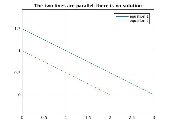
Plotting lines for linear system (ii)
Here the two lines are parallel and do not intersect since the linear system has no solution.
L1 = diag( b(1)./A(1,:) )              % two points satisfying eq.1
L2 = diag( b(2)./A(2,:) )              % two points satisfying eq.2

plotpoints(L1); hold on                % plot line for eq.1
plotpoints(L2,'--'); hold off          % plot line for eq.2
axis equal; grid on; title('The two lines are parallel, there is no solution')
legend('equation 1','equation 2')
L1 =
            3            0
            0          1.5
L2 =
     2     0
     0     1
Solving linear system (iii)
Since A is singular there is either no solution or infinitely many solutions.
Note that the backslash command in machine arithmetic gives a warning "matrix is singular to working precision". But it does not return any solution (despite the fact that there are solutions).
Using symbolic computation in Matlab we obtain a particular solution xpart, and a basis V for the null space (one vector). Hence the solution is given by a line xpart+t*V with arbitrary t.
b = [3;6]
% Using Matlab with machine arithmetic
x = A\b                                % Matlab gives NaN (not a number)
% Using symbolic computation:
xpart = sym(A)\sym(b)                  % symbolic \ gives one solution and
                                       % warning that more solutions exist
V = null(sym(A))                       % basis for null space
b =
     3
     6
Warning: Matrix is singular to working precision.
x =
   NaN
   NaN
Warning: The system is rank-deficient. Solution is not unique.
xpart =
 3
 0
V =
 -2
  1
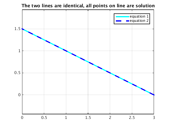
Plotting lines for linear system (iii)
Here the two lines are parallel and do not intersect since the linear system has no solution.
L1 = diag( b(1)./A(1,:) )              % two points satisfying eq.1
L2 = diag( b(2)./A(2,:) )              % two points satisfying eq.2

plotpoints(L1,'c','LineWidth',3); hold on    % plot line for eq.1
plotpoints(L2,'b--','LineWidth',3); hold off % plot line for eq.2
axis equal; grid on; title('The two lines are identical, all points on line are solution')
legend('equation 1','equation 2')
L1 =
            3            0
            0          1.5
L2 =
            3            0
            0          1.5