Solution Assignment 2 (MATH464, Spring 2020)
Contents
You need to download an m-file
Download the m-file foursum.m. Put it in the same folder as your other m-files.
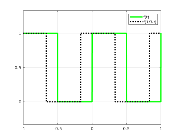
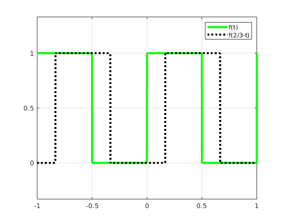
1(a) Sketch graphs of f(t) and f(1/3-t), graphs of f(t) and f(2/3-t)
(The vertical lines are not really part of the graphs.)
format compact; format short g
frac = @(x) x-floor(x);      % fractional part
f = @(x) frac(x)<.5;         % define function f

t = -1:.001:1;
plot(t,f(t),'g',t,f(1/3-t),'k:','LineWidth',3); axis equal
grid on; xticks(-1:.5:1); yticks(-1:.5:1);
legend('f(t)','f(1/3-t)')

snapnow

plot(t,f(t),'g',t,f(2/3-t),'k:','LineWidth',3); axis equal;
grid on; xticks(-1:.5:1); yticks(-1:.5:1);
legend('f(t)','f(2/3-t)')
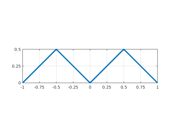
1(a)(iii) Sketch graph of q(x) on [-1,1]
We found: q(x) is 1-periodic function with
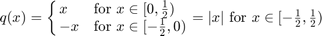
x = linspace(-1,1,1000);
q = abs(x-round(x));
plot(x,q,'LineWidth',3);
xticks(-1:.25:1); yticks(0:.25:.5); axis equal;  axis([-1 1 0 .5]); grid on
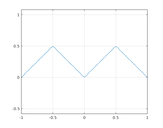
1(b) Plot  for convolution q=f*f
Note that  .
.
nv = 1:10;                   % vector of frequencies
qhpos = -1./(pi^2*nv.^2);    % vector qhpos = [qhat_1,...,qhat_{10}]
qhpos(2:2:end) = 0;          % set to zero for even k

x = linspace(-1,1,1000);     % 1000 equidistant points from -1 to 1 for plotting
plot(x,foursum(x,.25,qhpos)); grid on; axis equal
Warning: Imaginary parts of complex X and/or Y arguments ignored
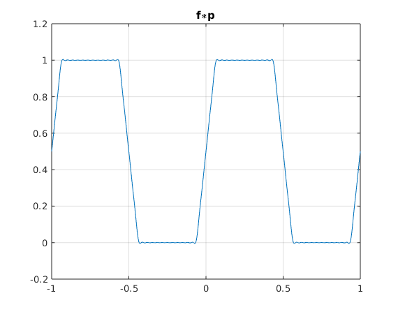
2(b) Plot  for h=1/8
Note  ,
,  .
.
h = 1/8;
nv = 1:30;
fh0 = .5;
fhpos = -1i./(pi*nv);        % vector fhpos = [qhat_1,...,qhat_{10}]
fhpos(2:2:end) = 0;          % set to zero for even k

ph0 = 1;
phpos = sinc(nv*h);          % NOTE: sinc_Matlab(x) = sinc(pi*x)

x = linspace(-1,1,1000);     % 1000 equidistant points from -1 to 1 for plotting
plot(x,foursum(x,fh0*ph0,fhpos.*phpos));
grid on; title('f{\ast}p')
Warning: Imaginary parts of complex X and/or Y arguments ignored
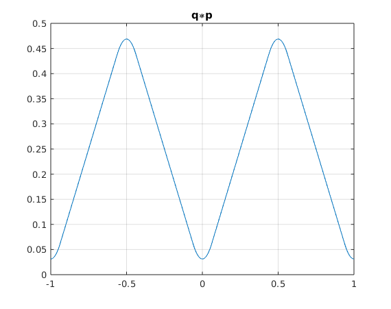
2(b) Plot 
Note , .
qh0 = fh0*fh0;
qhpos = fhpos.*fhpos;
plot(x,foursum(x,qh0*ph0,qhpos.*phpos));
grid on; title('q{\ast}p')
Warning: Imaginary parts of complex X and/or Y arguments ignored
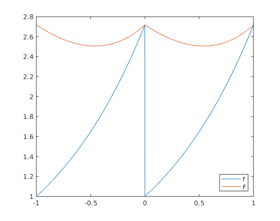
4(a)
Consider 1-periodic functions  with
with  and
and  for
for ![$x\in[0,1]$](a2sol_eq00029426888847692995.png) .
.
x = (0:999)/1000;
f = exp(x);
F = f + (exp(1)-1)*(1-x);
plot([x-1,x],[f,f],[x-1,x],[F,F])
legend('f','F','Location','SouthEast')
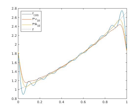
4(c),(d) Plot  together with
We have

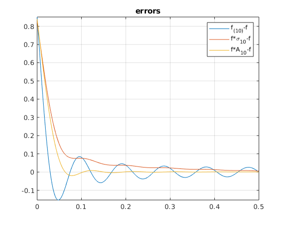
N = 10;
Nv = 1:N;
c = exp(1) - 1;
fh0 = c;
fhpos = c./(1-2i*pi*Nv);
shpos = (1-Nv/(N+1));     % f*sigma10: fhat_k*(1-|k|/(N+1))
qhpos = sinc(Nv/(N+.5));  % f*A10:     fhat_k*sinc_Matlab(k/(N+.5))

x = 0:.001:1;
plot(x,foursum(x,fh0,fhpos),x,foursum(x,fh0,fhpos.*shpos),...
     x,foursum(x,fh0,fhpos.*qhpos),x,exp(x),'k:')
legend('f_{(10)}','f*\sigma_{10}','f*A_{10}','f','Location','NorthWest')

snapnow
x = 0:.001:.5;
f = exp(x);
plot(x,foursum(x,fh0,fhpos)-f,x,foursum(x,fh0,fhpos.*shpos)-f,...
     x,foursum(x,fh0,fhpos.*qhpos)-f)
grid on; axis tight; title('errors')
legend('f_{(10)}-f','f*\sigma_{10}-f','f*A_{10}-f')
Warning: Imaginary parts of complex X and/or Y arguments ignored
Warning: Imaginary parts of complex X and/or Y arguments ignored
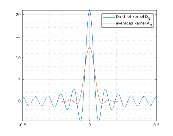
4(d) Plot Dirichlet kernel  , kernel
For  we have the Fourier coefficients
 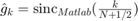 for
for  ,
,  for
for  .
.
Note that for ![$x\in[.25,.75]$](a2sol_eq06322394059567932196.png) we have
we have  with
with  . Therefore
  in [.25,.75], see problem 3(i).
x = -.5:.001:.5;
plot(x,foursum(x,1,Nv.^0),x,foursum(x,1,qhpos));
axis tight; grid on; grid minor
legend('Dirichlet kernel D_N','averaged kernel A_N')
Warning: Imaginary parts of complex X and/or Y arguments ignored