Examples for discrete Fourier transform from class (Sept. 25)

Contents

You need to download some f-files
Example 1: Convolution of discrete signals f,g
Example 2: For given signal f find best approximation p in T_5

You need to download some f-files

Download the following m-files and put them in the same directory with your other m-files:

four.m , ifour.m , fext.m , ftrunc.m

format compact        % don't print blank lines between results

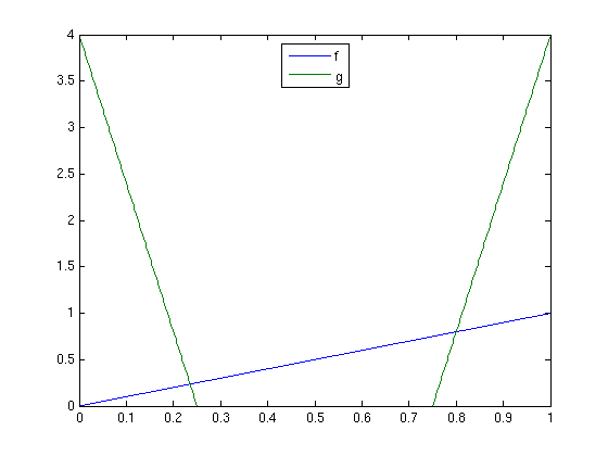
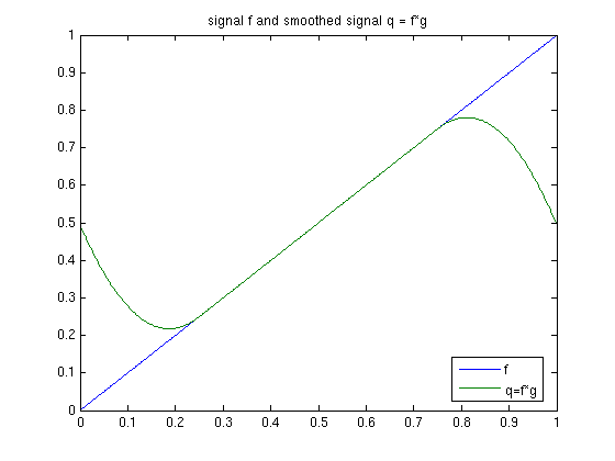
Example 1: Convolution of discrete signals f,g

Use the discrete Fourier transform to compute the convolution f*g.

N = 512;
x = (0:N-1)/N;
f = x;                                 % signal f
M = N/4;
g = 4*[M:-1:1,zeros(1,N-2*M),0:M-1]/M; % filter g (has integral 1, "local averaging")
figure(1); plot(x,f,x,g); legend('f','g','Location','best');

fh = four(f); gh = four(g);
qh = fh.*gh;
q = ifour(qh);
figure(2); plot(x,f,x,q); legend('f','q=f*g','Location','best');
title('signal f and smoothed signal q = f*g')

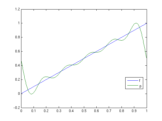
Example 2: For given signal f find best approximation p in T_5

We need to truncate the Fourier vector to length 11.

N = 512;
x = (0:N-1)/N;
f = x;                            % signal f
fh = four(f);
gh = ftrunc(fh,11);               % only coefficients for frequencies -5,...,5
ph = fext(gh,N);                  % extend with zeros for higher frequencies (for plotting)
p = ifour(ph);
plot(x,f,x,p); legend('f','p','Location','best')