Approximating the continuous Fourier transform fhat(xi) using the discrete Fourier transform (FFT)
Contents
You need to download some m-files
Download the following m-files and put them in the same directory with your other m-files:
format compact % don't print blank lines between results
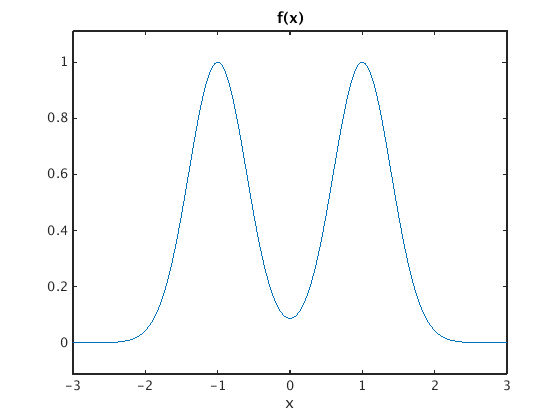
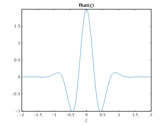
Define f(x) and find Fourier transform fhat(xi)
syms x xi                                    % set up symbolic variables
Pi = sym('pi');                              % and symbolic pi

f = exp(-Pi*(x-1)^2) + exp(-Pi*(x+1)^2)
fhat = simple(Four(f,x,xi))                  % find Fourier transform and simplify

figure(1); ezplot(f,[-3,3]); title('f(x)')   % plot f
figure(2); ezplot(fhat,[-2,2]); axis tight   % plot fhat
title('fhat(\xi)')
f =
exp(-pi*(x - 1)^2) + exp(-pi*(x + 1)^2)
fhat =
2*exp(-pi*xi^2)*cos(2*pi*xi)
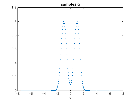
Take samples g_j = f(jh) for j=-M...M
h = 0.05;                                    % spacing
M = 150;
N = 2*M+1;                                   % number of values
X = (-M:M)*h;                                % discrete x values

g = exp(-pi*(X-1).^2) + exp(-pi*(X+1).^2);   % samples of f
plot(X,g,'.')                                % plot samples
xlabel('x'); title('samples g')
Find discrete Fourier transform
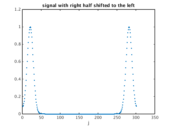
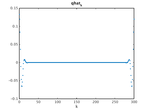
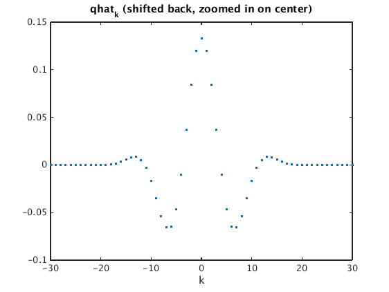
gs = ifftshift(g);                           % shift left half of signal to the right
figure(1); plot(gs,'.');
xlabel('j'); title('signal with right half shifted to the left')

qhat = four(gs);
figure(2); plot(0:N-1,qhat,'.');
xlabel('k'); title('qhat_k')

qhats = fftshift(qhat);                      % shift right half to the left
figure(3); plot(-M:M,qhats,'.');
xlim([-30 30]); xlabel('k')                  % show -30...30 on horizontal axis
title('qhat_k (shifted back, zoomed in on center)')
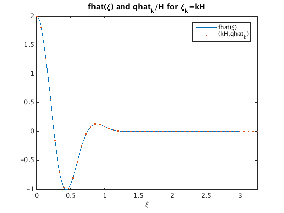
How is qhat related to fhat?
Answer: for H = 1/(N*h) we have that qhat_k/H approximates fhat(k*H)
H = 1/(N*h);                                 % spacing in frequency domain
ezplot(fhat,[0,3]); hold on                  % plot fhat
plot((0:49)*H,qhat(1:50)/H,'.');             % plot points (k*H,qhat_k)
hold off; axis tight
title('fhat(\xi) and qhat_k/H for \xi_k=kH')
legend('fhat(\xi)','(kH,qhat_k)')