Solving the Wave Equation (Dirichlet case) in 2 Dimensions using the Discrete Sine Transform
Contents
You first have to download m-files
Download the m-files sintr.m , isintr.m and put them in the same directory as your other m-files.
Solve the wave equation  in a rectangle
We have a rectangular rubber membrane which is fixed at the boundary. The vertical displacement is described by a function  for
for ![$x\in [0,A]$](wave2d_eq06895032831639178498.png) ,
, ![$y\in[0,B]$](wave2d_eq10287963619840255830.png) ,
,  .
.
We assume that the displacement is zero on all four sides of the rectangle (Dirichlet conditions). At time  the initial displacement
  and the initial velocity
  is given.
The function  satisfies the wave equation:

We have Dirichlet boundary conditions on all four sides of the rectangle for all  :
:


We write the solution  as a sine series with respect to both x and y: With
  and
and 

From this we get  and
and

This gives the following Solution Formula: First find the sine series of  and
and  with respect to both x and y:


Let  . Then the solution is given by
![$$ u(x,y,t) = \sum_{k=1}^\infty \sum_{\ell=1}^\infty \left[b_{k\ell} \cos(\rho_{k\ell}t) + \frac{c_{k\ell}}{\rho_{k\ell}}\sin(\rho_{k\ell}t) \right] \sin(\mu_k x)\sin(\nu_\ell y)$$](wave2d_eq16564025379478066721.png)
Example: For a rectangle with lengths  and
and  we are given the initial conditions
  and
and  where
where

A=3; B=2;                       % lengths of rectangle sides
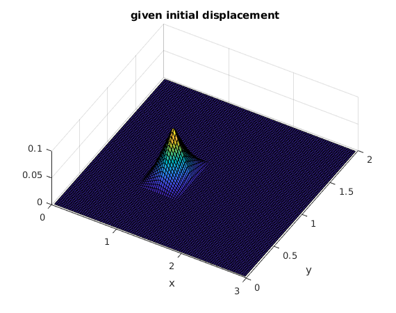
q = @(z) max(.3-abs(z),0);
f = @(x,y) q(x-1.1).*q(y-0.9);  % given function f(x,y) for initial condition

M = 100;                        % use spacing A/M for x
x = A*(1:M-1)/M;                % only interior nodes
N = 100;                        % use spacing B/N for y
y = B*(1:N-1)/N;                % only interior nodes

[X,Y] = ndgrid(x,y);            % X,Y are arrays of size M by N
F = f(X,Y);                     % F is array of values of f on grid:  F(j,k) = f(x_j,y_k)

surf(x,y,F');
view(30,70);
xlabel('x'); ylabel('y'); title('given initial displacement')
Use the discrete sine transform to compute the solution at several times
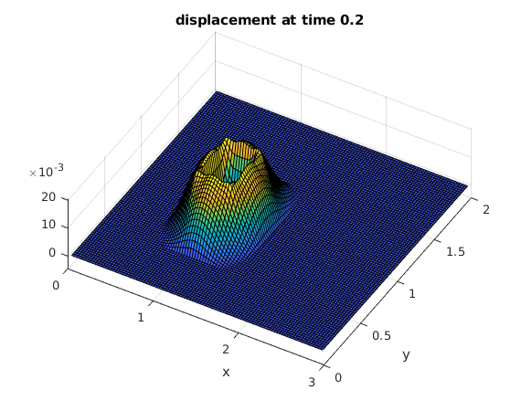
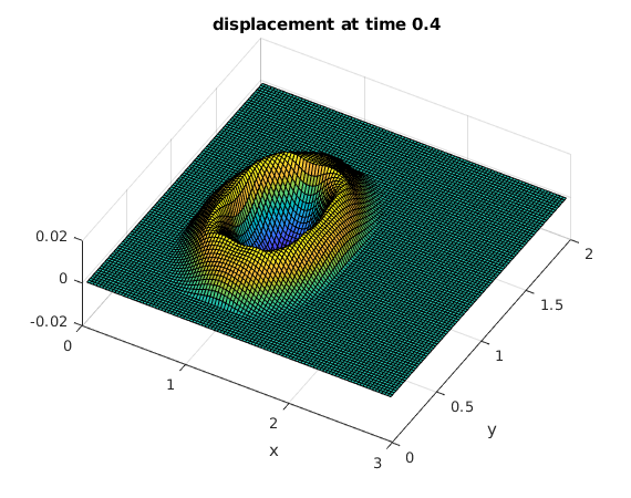
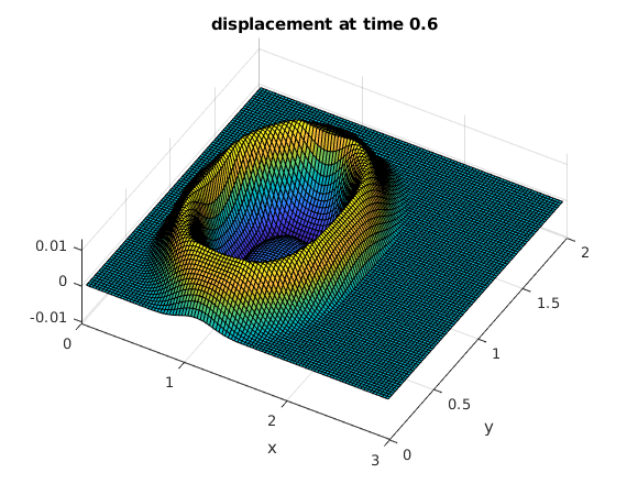
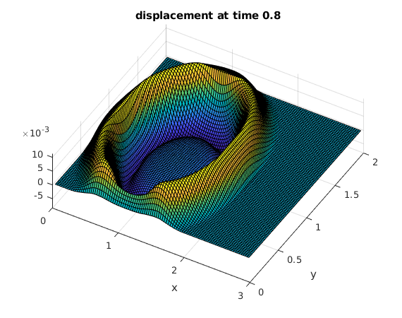
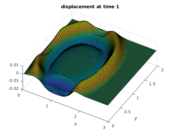
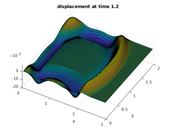
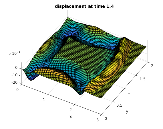
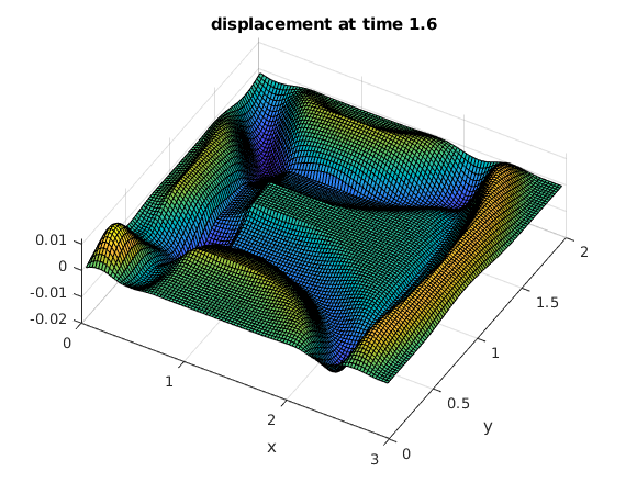
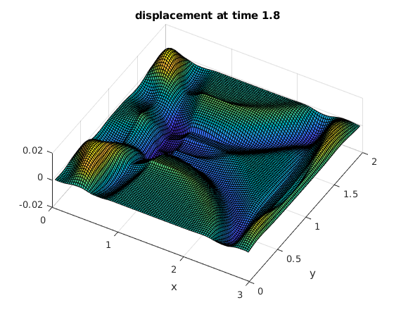
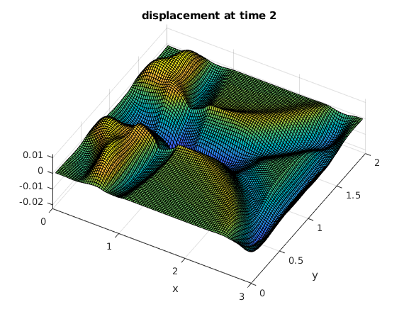
The initial peak causes an expanding circular wave. The waves are reflected at the four sides of the rectangle.
tv = .2:.2:2;                   % find solutions for these times

bx = sintr(F);                  % apply sine transform to columns
b = sintr(bx')';                % apply sine transform to rows

mu = (1:M-1)*pi/A;              % vector of mu_k
nu = (1:N-1)*pi/B;              % vector of nu_l
[Mu,Nu] = ndgrid(mu,nu);        % Mu,Nu are arrays of size M by N
rho = sqrt(Mu.^2+Nu.^2);        % rho from solution formula (array of size M by N)

for t=tv                        % for all times in vector tv
  C = b.*cos(rho*t);              % solution formula in frequency domain
  Cx = isintr(C')';               % apply inverse sine transform to rows
  U = isintr(Cx);                 % apply inverse sine transform to columns
  surf(x,y,U');                   % make surface plot of solution
  view(30,70);
  xlabel('x'); ylabel('y'); title(sprintf('displacement at time %g',t))
  snapnow                         % show current plot now
end
