[ts,ys] = ode45('f',[-2,2],1);
plot(ts,ys)

First write an m-file f.m for the function
f corresponding to the right hand side
of the differential equation y'(t) =
f(t,y(t)). E.g., for the differential
equation y'(t) = t
y(t)2 write an m-file f.m containing
function s = f(t,y)
s = t*y^2;
To find the numerical solution for
t going from t0 to T with the initial
condition y(t0)=y0 use
[ts,ys] = ode45('f',[t0,T],y0)
This gives a vector ts of t-values and a vector
ys of corresponding y-values.
The y-value at t=T is
ys(end), the last element of ys.
To plot the numerical solution use
plot(ts,ys).
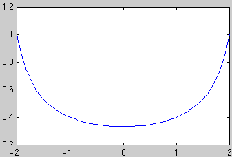
Example: To plot the solution of the initial value problem y'(t) = t y(t)2, y(-2)=1 in the interval [-2,2] use
[ts,ys] = ode45('f',[-2,2],1);

  plot(ts,ys)
To combine plots of several solution
curves use the commands hold on and
hold off: After obtaining the first plot type
hold on, then all subsequent commands plot in the same window.
After the last plot command type hold off.
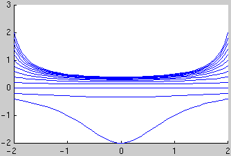
Example: Plot the 13 solution curves with the initial conditions y(-2) = -0.4, -0.2, ..., 1.8, 2:
hold on
for y0=-0.4:0.2:2
  [ts,ys] = ode45('f',[-2,2],y0); plot(ts,ys)
end
hold off

To obtain numerical values of the solution at
specific t values: You can specify a vector tv of t
values and use [ts,ys] = ode45(f,tv,y0). The
first element of the vector tv is the initial t value; the vector
tv must have at least 3 elements. E.g., to obtain the solution
with the initial condition y(-2)=1 at t = -2, -1.5, ..., 1.5, 2 and
display the results as a table with two columns, use
[ts,ys]=ode45('f',-2:0.5:2,1);

  [ts,ys]
Example problem: The angle y of a driven pendulum satisfies the differential equation
y''(t) = -sin(y(t)) + sin(5 t)
and the initial conditions
y(0) = 1
y'(0) = 0.
If your problem is of order 2 or higher: rewrite your problem as a first order system. Let y1=y and y2=y', this gives the first order system
y1' = y2,
y2' = -sin(y1) + sin(5 t)
with the initial conditions
y1(0) = 1
y2(0) = 0.
Write an m-file f.m for the right hand side of the
first order system: Note that f must be specified as a
column vector using [...;...]
(not a row vector using [...,...]). In the
definition of f, use y(1) for
y1, use y(2) for
y2. The file f.m should have the form
function s = f(t,y)expression for y1'
s = [;expression for y2'];
For our example the first component of f is
y2, the second component is -sin(y1) +
sin(5 t) and we use
function s = f(t,y)

s = [ y(2); -sin(y(1))+sin(5*t) ];
To find the numerical solution for
t going from t0 to T with initial values
y10 and y20 use
[ts,ys] = ode45('f',[t0,t1],[y10;y20])
Note that each row of the matrix ys contains 2 entries
corresponding to the two components of the solution at that time.
To plot the solution functions
y1(t) and y2(t) vs.
t use plot(ts,ys).
Example: For the driven pendulum problem from above we use
[ts,ys] = ode45('f',[0,20],[1;0]); % find ts, ys

  plot(ts,ys)                        % make plot of y1 and y2 vs. t


  [ts,ys]                 % show table with 3 columns for t, y1, y2
You can obtain the vector of y1 values in the first column of
ys by using ys(:,1), therefore
plot(ts,ys(:,1)) plots only
y1(t).
To obtain numerical values at specific
t values: You can
specify a vector tv of t values and use [ts,ys] =
ode45('f',tv,[y10;y20]). The first element of the vector
tv is the initial t value; the vector tv must have
at least 3 elements. E.g., to obtain the solution with the initial values
[1;0] at t = 0, 0.5, ..., 10 and display the results as a table
with 3 columns t, y1, y2,
use
[ts,ys]=ode45('f',0:0.5:10,[1;0]);

  [ts,ys]
To plot trajectories in the phase plane: To see the points with coordinates ( y1(t), y2(t) ) in the y1, y2 plane for t going from 0 to 20 use
Tobias von Petersdorff ,
[ts,ys] = ode45('f',[0,20],[1;0]);   % find ts, ys

  plot(ys(:,1),ys(:,2))              % make plot of y2 vs. y1
 tvp@math.umd.edu