Contents

Stability of First Order Initial Value Problems

% In this presentation we shall examine several first order
% ordinary differential equations
%       y' = f(t, y)

% and consider the stability of initial value problems
%       y' = f(t, y), y(t_0) = y_0

% associated with them. We shall see that small changes in
% initial data may or may not instigate substantial changes
% in the behavior of the solution as time (the independent
% variable t) progresses. Per Theorem 5.2 on p. 58 of
% Differential Equations with Matlab, 2nd ed, by Hunt et al
% aka HOLR, we know that the sign of the partial of f wrt y
% is the determining factor.

% We shall consider problems for
% which we can find a formula solution of the original
% equation, as well as examples in which we cannot find a
% formula solution and we must work numerically or
% graphically.

% Our examples will illustrate Theorem 5.2 and the succeeding
% discussion on p. 58 of HOLR. Stated succinctly, the Theorem
% asserts, in its simplest interpretation, that in regions
% where the partial derivative of f with respect to y is
% negative, the related initial value problems will be stable,
% and in regions where the partial is positive, associated
% IVPs will be unstable.
% Let's see.

clear all
close all

A stable example in which we can find a formula solution

% Let us consider the first order linear equation
%       ty' + y = t cos(t).

% Solving for y', we can also write the equation as
%       y' = -(1/t)y + cos(t).    [1]

% In this form we see that there is a singularity at t = 0,
% and so we will have to consider regions that do not include
% any portion of the y-axis. In fact, since we are thinking
% of t as time, we will restrict our attention to t > 0.

% Next, let's note that the partial derivative of the right
% side of equation [1] wrt y is -1/t, which is negative for
% all t > 0. So Theorem 5.2 predicts stability. Let's see.

% First let's find the general solution.
% Note: I name the output, which is good practice, since I
% might need to use it later.
gensol1 = dsolve('t*Dy + y = t*cos(t)', 't')

 
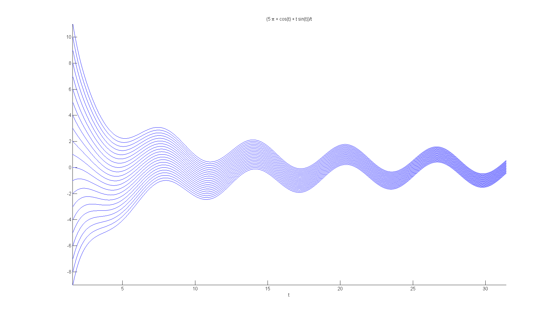
gensol1 =
 
(C2 + cos(t) + t*sin(t))/t
 

Matlab handles the equation easily and produces a formula solution that makes transparent the singularity at t = 0.

% Next, let's consider the IVP
%       ty' + y = t cos(t), y(pi/2) = 1.

% Matlab solves it as follows:
ivp1a = dsolve('t*Dy + y = t*cos(t)', 'y(pi/2) = 1', 't')

 
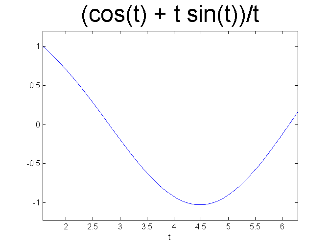
ivp1a =
 
(cos(t) + t*sin(t))/t
 

A sinusoidal superimposed on a damped sinsusoidal. Let's graph it, first on a relatively short interval, then a longer one.

ezplot(ivp1a, [pi/2 2*pi])
set(get(gca, 'Title'),'Fontsize', 30)
figure; ezplot(ivp1a, [pi/2 10*pi])
set(get(gca, 'Title'),'Fontsize', 30)

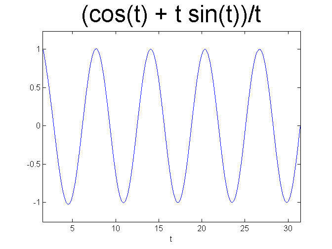
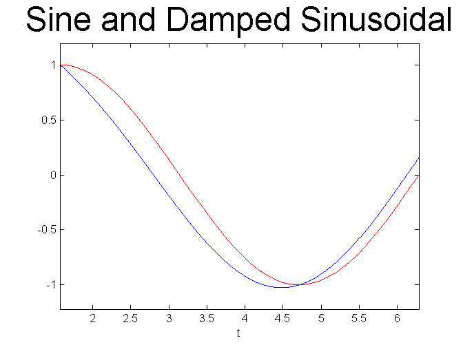
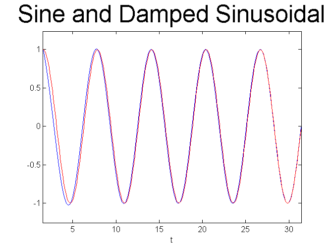
The solution looks like a plain sine wave, that is, the damped sinusoidal is masked. So let's compare to see the difference.

% Compare with a sine curve
close all
ezplot(ivp1a, [pi/2 2*pi])
hold on, X=pi/2:0.1:2*pi;plot(X, sin(X), 'r')
title('Sine and Damped Sinusoidal', 'FontSize', 30)
figure; ezplot(ivp1a, [pi/2 10*pi])
hold on, X=pi/2:0.1:10*pi;plot(X, sin(X), 'r')
title('Sine and Damped Sinusoidal', 'FontSize', 30)

% For large t, the term cos(t)/t is very small and so the
% solution curve given by the formula sin(t) + cos(t)/t is
% extremely close to just sin(t).

Now let's perturb the initial data and see what happens to the solution as t grows. Instead of y(pi/2) = 1, let's consider y(pi/2) = 1 + epsilon

ivp1b = dsolve('t*Dy + y = t*cos(t)', 'y(pi/2) = 1 + epsilon', 't')

 
ivp1b =
 
(cos(t) + (pi*epsilon)/2 + t*sin(t))/t
 

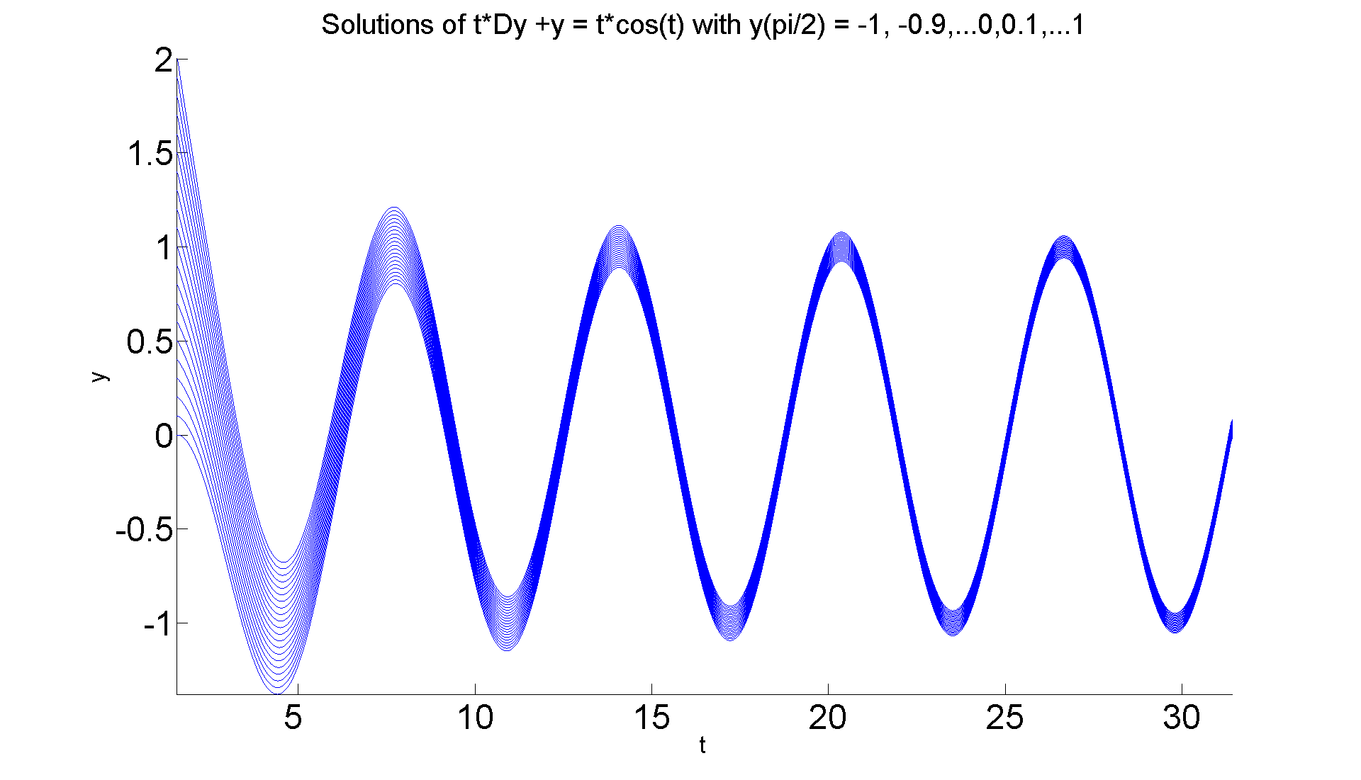
Next we'll graph the solutions for very small choices of epsilon, and then for moderately large choices of epsilon. Our goal is to see how these solutions differ from the original as t grows.

figure; set(gcf, 'Position', [1 1 1920 1420])
hold on
for eps = -1:0.1:1
    ezplot(subs(ivp1b, 'epsilon', eps), [pi/2 10*pi])
end
axis tight
title ('Solutions of t*Dy +y = t*cos(t) with y(pi/2) = -1, -0.9,...0,0.1,...1','FontSize', 25)
        xlabel ('t', 'FontSize', 20), ylabel ('y', 'FontSize', 20)
set(gca,'XTickLabel',get(gca, 'XTickLabel'),'FontSize',30)
hold off

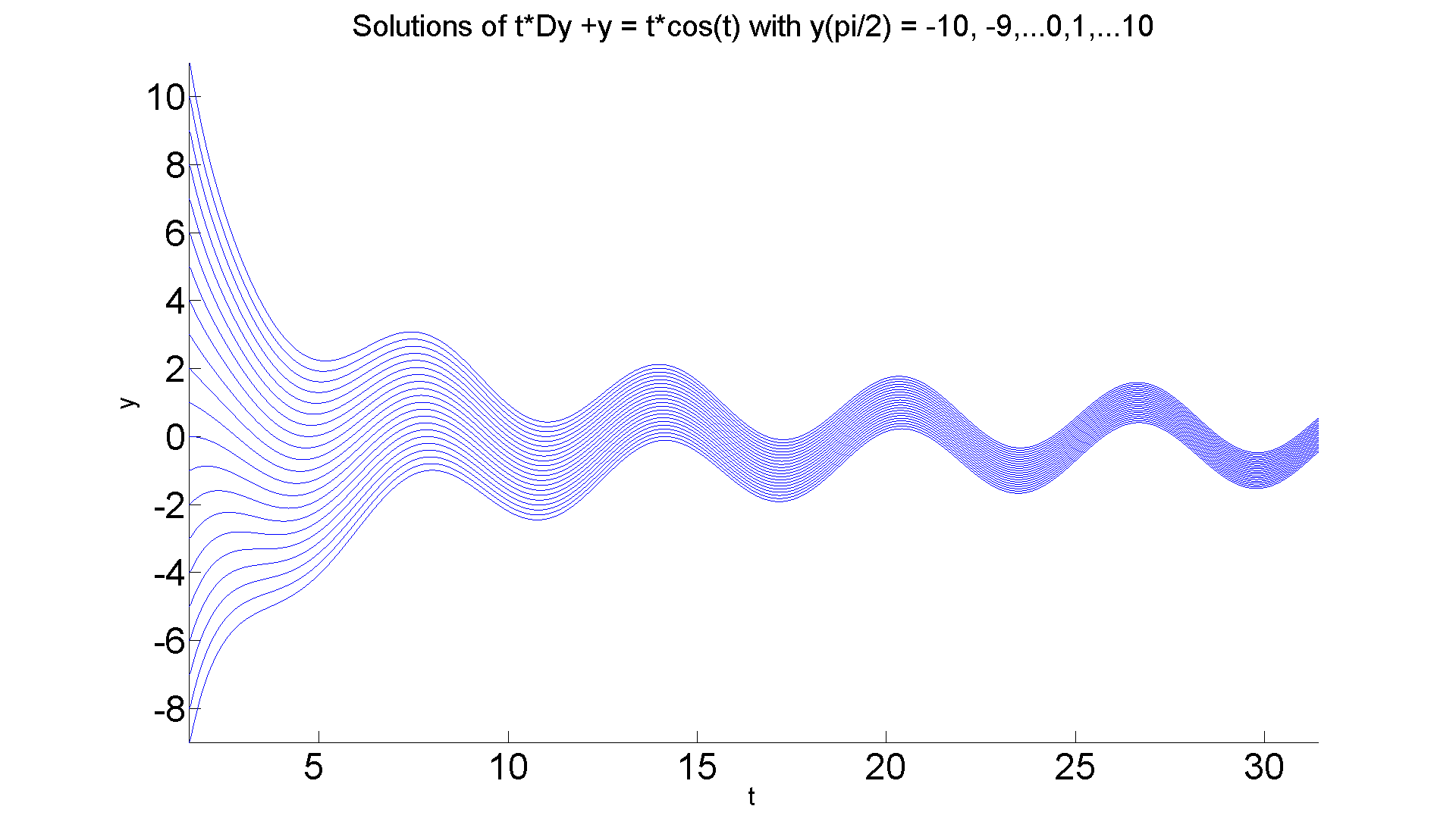
Now the wider initial data.

figure;  set(gcf, 'Position', [1 1 1920 1420])
hold on
for eps = -10:10
    ezplot(subs(ivp1b, 'epsilon', eps), [pi/2 10*pi])
end
axis tight
title ('Solutions of t*Dy +y = t*cos(t) with y(pi/2) = -10, -9,...0,1,...10','FontSize', 25)
    xlabel ('t', 'FontSize', 20), ylabel ('y', 'FontSize', 20)
set(gca,'XTickLabel',get(gca, 'XTickLabel'),'FontSize',30)
hold off

% The visual evidence of stability is very strong. In fact,
% this example illustrates a phenomenon we call asymptotic
% stabilty--not only do small perturbations of the initial
% data not result in much deviation from the original, but
% in fact the perturbed solutions tend toward the
% original as time increases.

Just for emphasis we'll make a movie as we step through the values of epsilon to further emphasize the stability.

figure; set(gcf, 'Position', [1 1 1920 1420])
hold on
for eps = -10:10
    ezplot(subs(ivp1b, 'epsilon', eps), [pi/2 10*pi])
    axis([pi/2 10*pi -9 11])
    M(11+eps)=getframe;
end
hold off

Stability of a 1st order IVP w/o a formula solution

clear all
close all

Now let us consider a first order linear equation, but with more complicated coefficients. ty' + (e^t)y = t cos(t). [2]

% Solving for y', we can rewrite the equation as
%       y' = -(1/t)(e^t)y + cos(t).

% Once again, there is a singularity at t = 0, and so
% we restrict our attention to t > 0.
% And as in equation [1], the relevant partial, -(1/t)(e^t),
% is always negative when t > 0, so we again expect stability.

% But let's see what happens if we try to find a general
% solution using dsolve.

gensol2 = dsolve('t*Dy + exp(t)*y = t*cos(t)', 't')

% Ughh! Matlab can't find a closed formula solution. It gives an
% answer in terms of a special function and an integral that it
% cannot evaluate. If you try to specify an initial value and use
% ezplot, Matlab cannot cope. So we
% will proceed as in DEwM, Chapter 6, that is, find a
% graphical solution. We shall delay to the next presentation
% the consideration of numerical solutions of equations for
% which we cannot find formula solutions.

 
gensol2 =
 
C2/exp(Ei(t)) + int(exp(Ei(t))*cos(t), t, IgnoreAnalyticConstraints)/exp(Ei(t))
 

Graphical Solution of Equation [2]

[T, Y] = meshgrid(0.5:0.2:5, -1:0.1:1);
S = -(1./T).*exp(T).*Y + cos(T);
L = sqrt(1 + S.^2);
quiver(T, Y, 1./L, S./L, 0.5), axis tight
title ('Direction field for t*dy/dy + exp(t)*y = t*cos(t)', 'FontSize', 20)
xlabel ('t', 'FontSize', 20)
ylabel ('y', 'FontSize', 20)

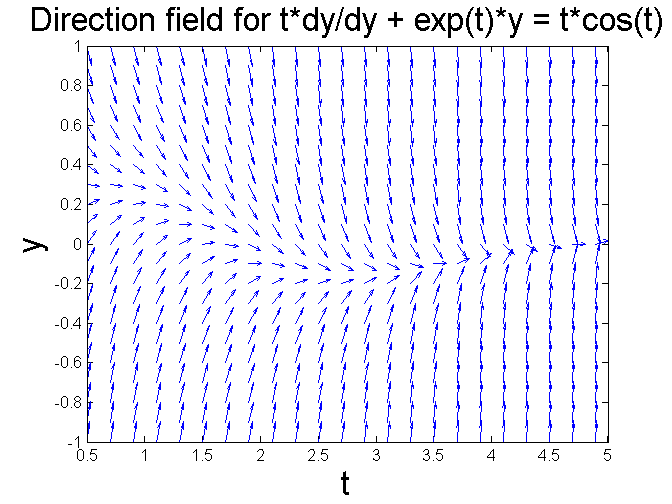
The behavior looks very much like the last example, although the stability seems to be even more dramatic, as the solution curves seem to tend toward a stable solution very quickly. But it's rather unclear from the graph as to the exact nature of the stable solution. Let's change the coordinates a little to see whether we can improve the picture and highlight the stable solution more clearly.

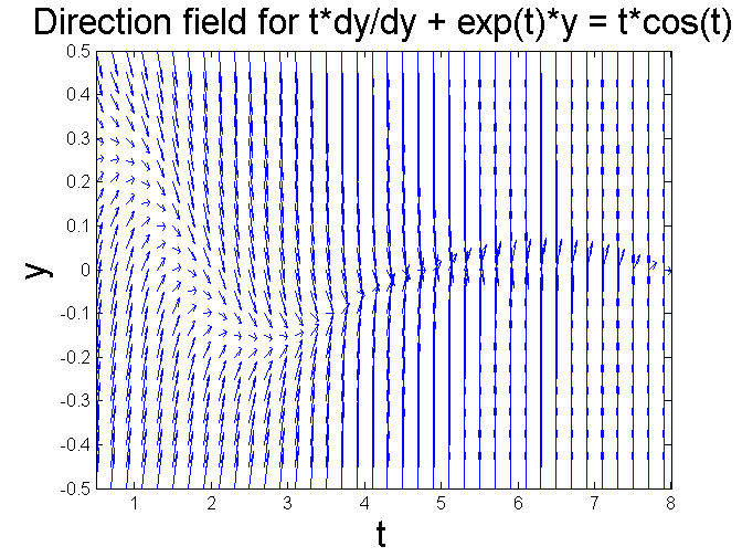
figure; [T, Y] = meshgrid(0.5:0.2:8, -0.5:0.05:0.5);
S = -(1./T).*exp(T).*Y + cos(T);
L = sqrt(1 + S.^2);
quiver(T, Y, 1./L, S./L, 0.5), axis tight
xlabel ('t', 'FontSize', 20), ylabel ('y', 'FontSize', 20)
title ('Direction field for t*dy/dy + exp(t)*y = t*cos(t)', 'FontSize', 20)

% The asymptotically stable solution looks like an oscillatory
% curve about the origin. In fact it is hard to see without
% using a numerical solution (as we will do in the next
% presentation). But in fact it is a damped oscillation.
% Can you explain from the differential equation itself
% (reproduced below) why
% the solution curves must decay to zero?

 %       ty' + (e^t)y = t cos(t)

Change of coefficient

% Now we'll change exp(t) to exp(-t) in the coefficient and
% examine the result.
figure; [T, Y] = meshgrid(0.5:0.2:5, -1:0.1:1);
S = -(1./T).*exp(-T).*Y + cos(T);
L = sqrt(1 + S.^2);
quiver(T, Y, 1./L, S./L, 0.5), axis tight
xlabel ('t', 'FontSize', 20), ylabel ('y', 'FontSize', 20)
title ('Direction field for t*dy/dy + exp(-t)*y = t*cos(t)', 'FontSize', 20)

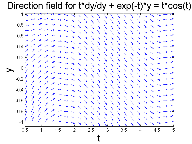
We still have stability, but all the solutions look like sinusoidals. Can you explain directly from the differential equation why that is so? ty' + (e^(-t))y = t cos(t)

% Note that these examples illustrate
% the difference between stability and asymptotic stability.
% In the former, small changes in the initial data
% result in only small changes in the solution as time
% increases, but in the latter, small changes in initial data
% result in essentially NO change over the long term as nearby
% solutions converge to the equilibrium solution, a
% phenomenon we have examined previously for autonomous
% equations.

An example of a non-stable solution

Simple alterations in a differential equation can make a huge difference in the behavior of the equation's solutions. Consider the following equation: ty' - y = t^2 cos(t).

% This is very similar to our original example, except that
% the sign preceding the 'y' term is now negative instead of
% positive, and the multiplier of cos(t) is now t^2 instead
% of t. Of course this means that when you solve the equation
% for y' and take the partial wrt y, the result becomes
% positive instead of negative and should lead to
% instability. We'll use Matlab to verify that. (Incidentally,
% the change from t to t^2 is really minor--I did it to make
% life easier on Matlab's symbolic solver; it is the change
% from y to -y that causes the major change in stability.
% Recall Theorem 5.2 to see why.

clear all
close all

gensol3 = dsolve('t*Dy - y = t^2*cos(t)', 't')

% Well that turned out to be pretty simple: t*sin(t) plus a
% linear term in t. Let's proceed as we did in the original
% case--that is, first specify an IVP corresponding to this
% equation; graph it over several intervals;
% then let the initial value vary; and finally see what
% happens to the corresponding solutions as t grows.
% Theorem 5.2 predicts instability.

 
gensol3 =
 
C2*t + t*sin(t)
 

Here's the initial vaue problem. ty' - y = t^2 cos(t), y(pi) = 0.

% Matlab solves it as follows
ivp3a = dsolve('t*Dy - y = t^2*cos(t)', 'y(pi) = 0', 't')

 
ivp3a =
 
t*sin(t)
 

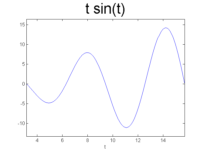
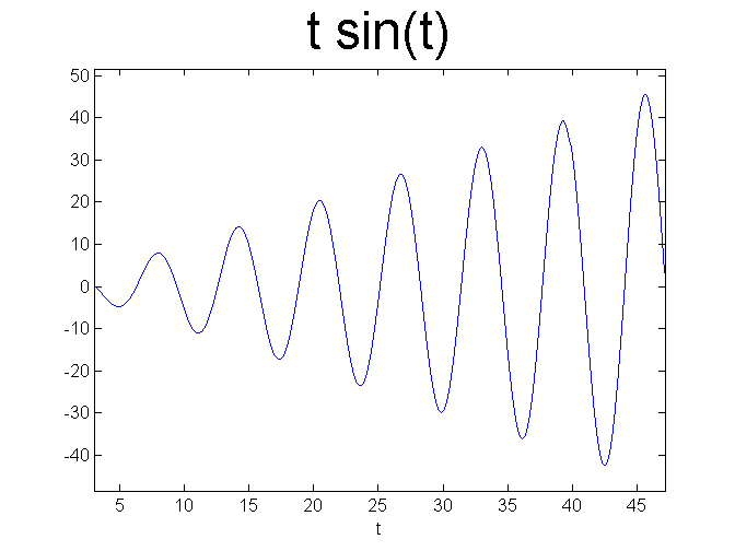
Next, let's graph the solution, as before over a shorter and then a longer interval.

ezplot(ivp3a, [pi 5*pi])
set(get(gca, 'Title'),'Fontsize', 30)
figure; ezplot(ivp3a, [pi 15*pi])
set(get(gca, 'Title'),'Fontsize', 30)

% We observe a sinusoidal, but with increasing amplitude.
% Now it should be clear from the general solution that no
% other solution is purely sinusoidal because of the linear
% term, and because of that term, the solutions correspondng
% to slightly perturbed intial data will move away from the
% solution we have just identified.
% Let's ilustrate that.

ivp3b = dsolve('t*Dy - y = t^2*cos(t)', 'y(pi) = epsilon', 't')

 
ivp3b =
 
t*sin(t) + (epsilon*t)/pi
 

figure;  set(gcf, 'Position', [1 1 1920 1420])
hold on
for eps = -1:0.25:1
    ezplot(subs(ivp3b, 'epsilon', eps), [pi 10*pi])
end
axis tight
title('Solutions of t*Dy - y = t^2*cos(t) with y(pi) = -1, -3/4,...0,1/4,...1', 'FontSize',25)
    xlabel('t', 'FontSize', 20); ylabel('y', 'FontSize', 20)
set(gca,'XTickLabel',get(gca, 'XTickLabel'),'FontSize',30)
hold off

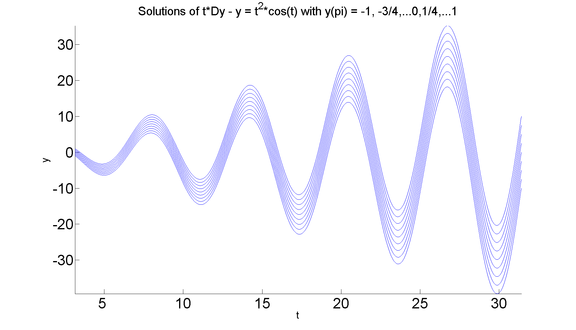
If you look carefully, you will see that out around t=25, the curves differ by as much as 20 units. But let's look out at a longer time interval as the divergence is slow.

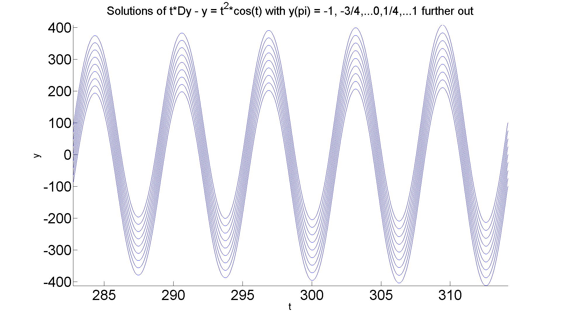
figure; set(gcf, 'Position', [1 1 1920 1420])
hold on
for eps = -1:0.25:1
    ezplot(subs(ivp3b, 'epsilon', eps), [90*pi 100*pi])
end
axis tight
title ('Solutions of t*Dy - y = t^2*cos(t) with y(pi) = -1, -3/4,...0,1/4,...1 further out','Fontsize', 25)
    xlabel('t','FontSize', 20); ylabel('y','FontSize', 20)
set(gca,'XTickLabel',get(gca, 'XTickLabel'),'FontSize',30)
hold off

% You must look carefully at the coordinates on the vertical
% axis to see that the curves on either end of the epsilon
% range are a couple hundred units apart, whereas they
% started less than two units apart.

A Mixed example

Now let's look at a final example in which the solutions exhibit mixed behavior with regard to stability.

%       y' = y*(1 - 2bt)

% where b is a very small positive number.
% Note that the partial of the right side with respect to y is
%       (1-2bt).

% That expression is positive when
%       t < 1/2b
% and negative when
%       t > 1/2b.

% Therefore according to the stability theorem, initial value
% problems in the former interval should be unstable, whereas
% those with initial data in the latter should be stable. Let's see.

% dsolve can handle this equation rather easily (it is both
% linear and separable). Let's solve it symbolically
% while imposing the initial condition
%       y(0) = 1 + d

% where you should think of d as also a small positive number.
clear all
close all
ivp4a = dsolve('Dy = y*(1 - 2*b*t)', 'y(0) = 1 + d', 't')

 
ivp4a =
 
(d + 1)/exp(b*t^2 - t)
 

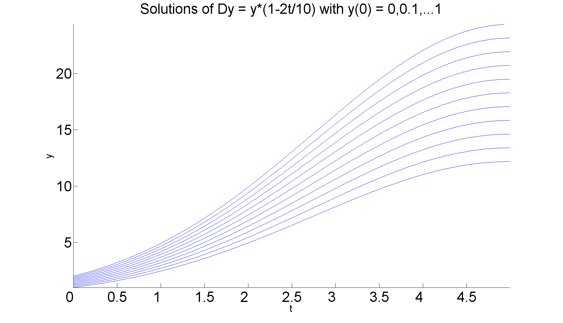
Now as t progresses from t = 0 to t = 1/2b, which you should think of as a big number, instability predicts that the solution curves for d > 0 move sharply away from that corresponding to d = 0. Here are the curves in case b = .1:

figure;
hold on
for k = 0:0.1:1
    ezplot(subs(ivp4a, {'b', 'd'}, [0.1 k]), [0 5])
end
axis tight
title ('Solutions of Dy = y*(1-2t/10) with y(0) = 0,0.1,...1','FontSize', 30)
        xlabel ('t', 'FontSize', 20), ylabel ('y', 'FontSize', 20)
set(gca,'XTickLabel',get(gca, 'XTickLabel'),'FontSize',30)
hold off
set(gcf, 'Position', [1 1 1920 1420])

% You can see the curves moving away from each other.

Here is more dramatic evidence with b one-tenth the size.

figure;
hold on
for k = 0:0.1:1
    ezplot(subs(ivp4a, {'b', 'd'}, [0.01 k]), [0 50])
end
axis tight
title ('Solutions of Dy = y*(1-2t/100) with y(0) = 0,0.1,...1','FontSize', 30)
        xlabel ('t', 'FontSize', 20), ylabel ('y', 'FontSize', 20)
set(gca,'XTickLabel',get(gca, 'XTickLabel'),'FontSize',30)
hold off
set(gcf, 'Position', [1 1 1920 1420])

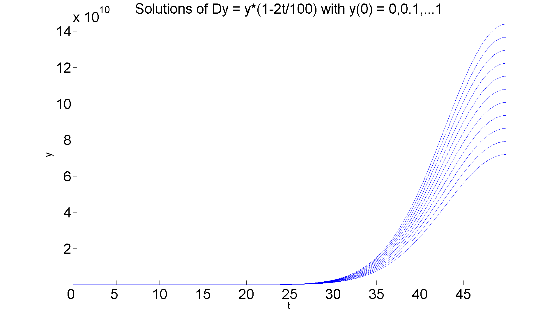
But now when we pass to the second interval, i.e., t > 1/2b, then the situation becomes stable. We can illustrate that by just extending the previous graphs.

figure;
hold on
for k = 0:0.1:1
    ezplot(subs(ivp4a, {'b', 'd'}, [0.1 k]), [0 10])
end
axis tight
title ('Solutions of Dy = y*(1-2t/10) over a longer interval','FontSize', 30)
        xlabel ('t', 'FontSize', 20), ylabel ('y', 'FontSize', 20)
set(gca,'XTickLabel',get(gca, 'XTickLabel'),'FontSize',30)
hold off
set(gcf, 'Position', [1 1 1920 1420])

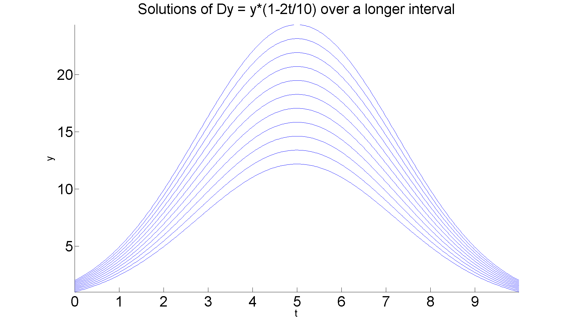
Even for smaller values of b, the same behavior is evident:

figure;
hold on
for k = 0:0.1:1
    ezplot(subs(ivp4a, {'b', 'd'}, [0.01 k]), [0 100])
end
axis tight
title ('Solutions of Dy = y*(1-2t/100) on a longer interval','FontSize', 30)
        xlabel ('t', 'FontSize', 20), ylabel ('y', 'FontSize', 20)
set(gca,'XTickLabel',get(gca, 'XTickLabel'),'FontSize',30)
hold off
set(gcf, 'Position', [1 1 1920 1420])

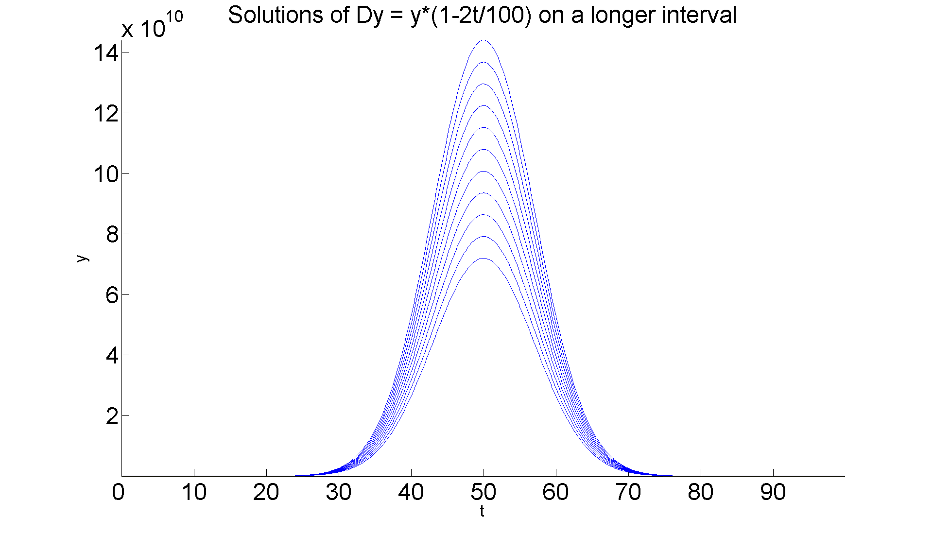
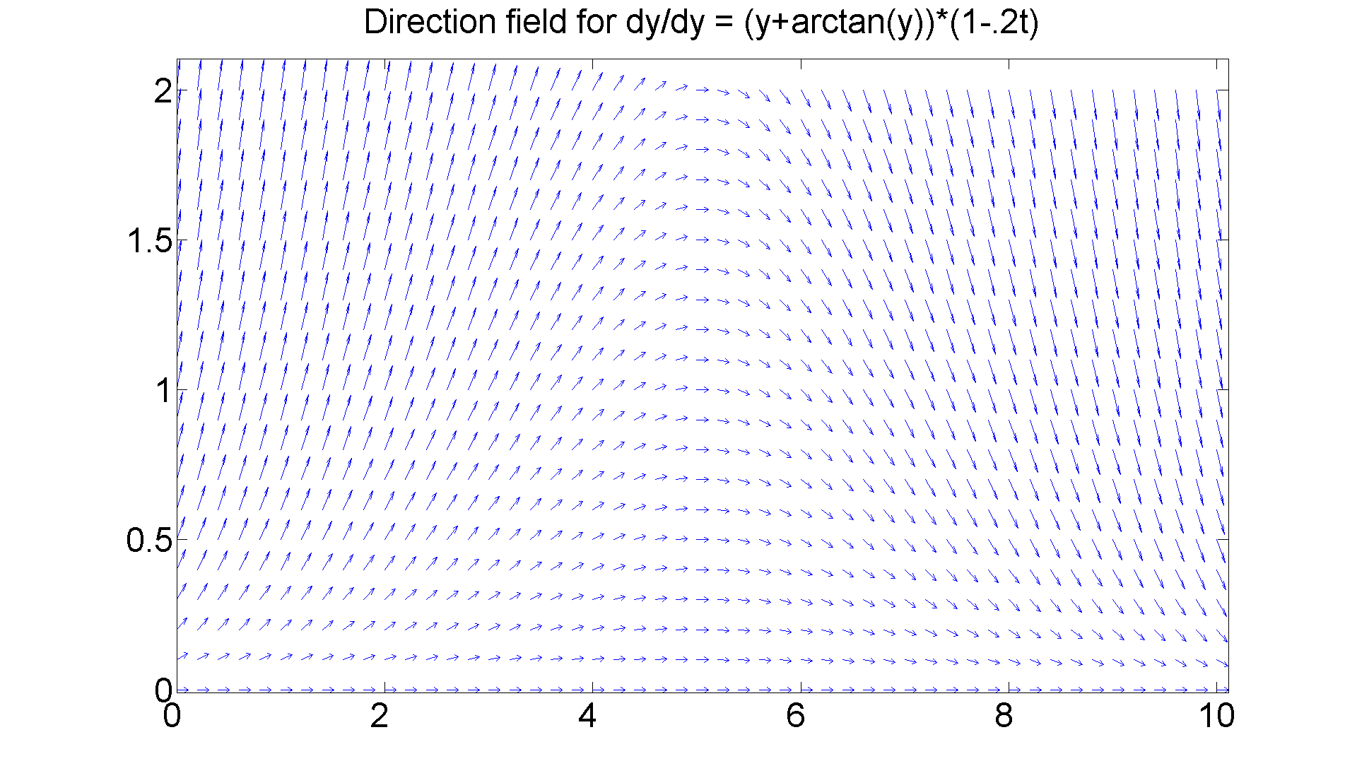
Lastly, this behavior has nothing to do with the fact that we can find a formula solution. Consider instead y' = (y+arctan(y))*(1 - 2bt).

% The partial will be
%       (1+1/(1+y^2))(1-2bt)

% and since the expression in y is always positive, the same
% analysis as in the previous case obtains. Since we cannot
% solve symbolically (try it, dsolve chokes on the equation),
% we draw the direction field for b = 0.1.

figure;
[T, Y] = meshgrid(0:0.2:10, 0:0.1:2);
S = (Y+ atan(Y)).*(1-0.2.*T);
L = sqrt(1 + S.^2);
quiver(T, Y, 1./L, S./L, 0.5), axis tight
title ('Direction field for dy/dy = (y+arctan(y))*(1-.2t)', 'FontSize', 30)
set(gca,'XTickLabel',get(gca, 'XTickLabel'),'FontSize',30)
set(gcf, 'Position', [1 1 1920 1420])

% We see essentially the same behavior as in the preceding case.

Published with MATLAB® 7.13