Contents
Numerical and Graphical Methods for 1st Order Equations
% Thus far we have studied first order ordinary differential
% equations for which we can find a symbolic or formula
% solution. Years ago, that is largely all that was done in
% a sophomore-level ODE course. But this masked the fact
% that, indeed, most ODEs cannot be solved symbolically.
% Just to illustrate that fact, consider the simple equation

%           y' + y = t.

% This equation is solved symbolically rather easily. But
% let us change it slightly by introducing a parameter.
% Consider now the equation

%           y' + y^b = t,

% where b is a real number. In fact it would not take you
% long to discover that Matlab can solve this equation only
% in case b = 0, 1, or 2. For no other values of b,
% positive or negative, can Matlab produce a formula
% solution of this differential equation. Nevertheless,
% situations arise in which we need to be able to say
% something about solutions to equations like this. In this
% course we develop two techniques for doing so:
% graphical and numerical. (Actually, as you have seen, we also
% develop some qualitative techniques, but they are much more
% ad hoc than the algebraic, graphical and numerical techniques
% that you will encounter.)

% For the purposes of illustration, we shall consider three
% examples:
%       b = 1, 1/2 and -2.

% The first example Matlab can solve of course, but not the
% other two. For the record, we'll try them; Matlab reports
% its failure in the second example, but just hangs in the
% third.
clear all
close all
dsolve('Dy + y = t', 't')
ans =

t + C3/exp(t) - 1
dsolve('Dy + sqrt(y) = t', 't')
Warning: Explicit solution could not be found.

ans =

[ empty sym ]
dsolve('Dy + 1/y^2 = t', 't') Oops, the % is there to remind me not to even try; take my word, it just hangs.
Direction Fields
You have learned the direction field method for first order equations y' = f(t, y).
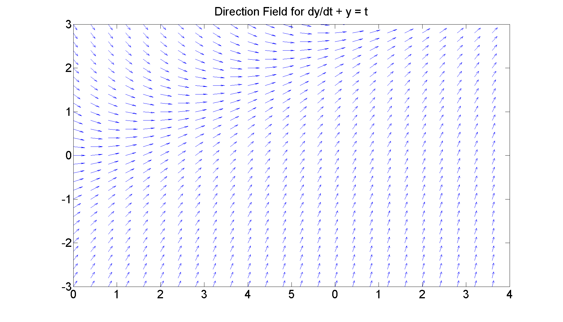
% If one draws a small vector at the point (t_0, y_0)
% having slope f(t_0, y_0), then one knows that the solution
% curve to the differential equation that passes through
% (t_0, y_0) must have slope = f(t_0, y_0) there. If we draw
% lots of such small slope line segments, then we get a
% global picture of the solution curves to the
% differential equation, which we have called the
% Direction Field of the equation. Naturally, Matlab can do
% this much better than we can freehand. So here are the
% direction fields for the three examples in question:
clear all
close all
figure;
[T, Y] = meshgrid(0:0.2:5, -3:0.2:3);
S = -Y + T;
L = sqrt(1 + S.^2);
quiver(T, Y, 1./L, S./L, 0.5), axis ([0 5, -3 3])
title 'Direction Field for dy/dt + y = t'
set(get(gca, 'Title'),'Fontsize', 25)
set(gca,'XTickLabel',get(gca, 'XTickLabel'),'FontSize',25)
set(gcf, 'Position', [1 1 1920 1220])
figureforbis1 = gcf

% The last command will allow me to recall this figure later.
% You can see the linear solution y = t - 1. The other
% solutions are obtained by adding a constant times
% exp(-t) to it.
figureforbis1 =

     1
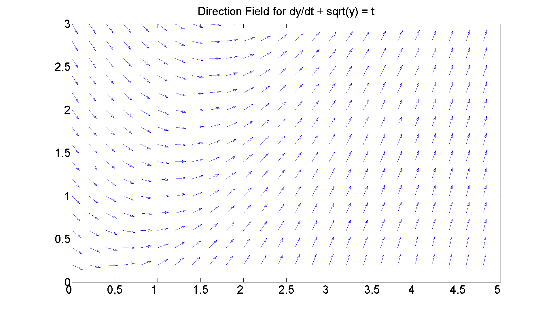
Now the first of the two equations for which we cannot find a formula solution. Since we are taking the square root of y, it behooves us to restrict y to positive values.
figure; set(gcf, 'Position', [1 1 1920 1420])
[T, Y] = meshgrid(0:0.2:5, 0.2:0.2:3);
S = -sqrt(Y) + T;
L = sqrt(1 + S.^2);
quiver(T, Y, 1./L, S./L, 0.5), axis([0 5, 0 3])
title 'Direction Field for dy/dt + sqrt(y) = t'
set(get(gca, 'Title'),'Fontsize', 25)
set(gca,'XTickLabel',get(gca, 'XTickLabel'),'FontSize',25)

% Gee it looks sort of similar to the first case. You have
% to look closely to see that the line y = t -1 is not
% really a solution. Let's refine the parameters a little
% to see that better.
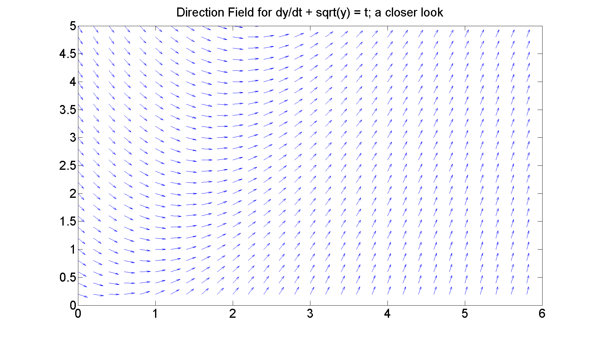
figure; set(gcf, 'Position', [1 1 1920 1420])
[T, Y] = meshgrid(0:0.2:6, 0.2:0.2:5);
S = -sqrt(Y) + T;
L = sqrt(1 + S.^2);
quiver(T, Y, 1./L, S./L, 0.5), axis([0 6, 0 5])
title 'Direction Field for dy/dt + sqrt(y) = t; a closer look'
set(get(gca, 'Title'),'Fontsize', 25)
set(gca,'XTickLabel',get(gca, 'XTickLabel'),'FontSize',25)
figureforbisonehalf = gcf

% The non-linearity is somewhat clearer now.
% Still, all the solutions seem to be squeezing together as
% time increases. We'll see that more clearly when we
% generate a numerical solution below.

% Here's an exercise for you:
% Show that
%       y = (1/4)t^2

% solves the equation. That is the limiting behavior of all
% the solution curves. But Matlab cannot figure that out
% on its own.
figureforbisonehalf =

     3
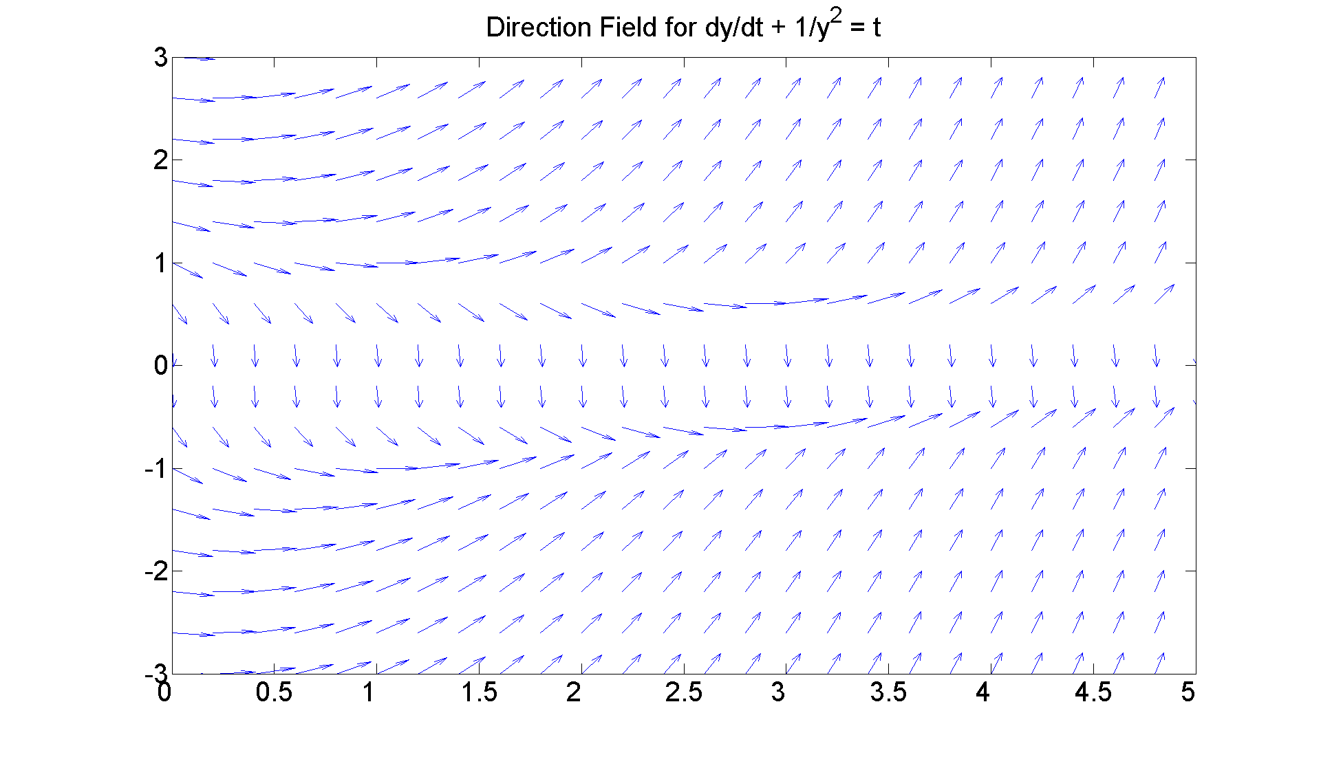
And now let's look at the third case on which Matlab's symbolic solver completely chokes. Since y appears in the denominator of the equation, we had better avoid y = 0.
figure; set(gcf, 'Position', [1 1 1920 1420])
[T, Y] = meshgrid(0:0.2:5, -3:0.4:3);
S = -1./Y.^2 + T;
L = sqrt(1 + S.^2);
quiver(T, Y, 1./L, S./L, 0.5), axis([0 5, -3 3])
title 'Direction Field for dy/dt + 1/y^2 = t'
set(get(gca, 'Title'),'Fontsize', 25)
set(gca,'XTickLabel',get(gca, 'XTickLabel'),'FontSize',25)

% Well we can clearly see the problem across the line y = 0.
% Perhaps I have been too clever by choosing the step size =
% 0.4 so that I would miss y = 0 in the computations. But
% there clearly is a problem. Above the t-axis, the solution
% curves come down then seem to go up off to
% infinity. Below the t-axis, the solution curves also come
% down initially, but then they seem to be
% crashing into the t-axis--but perhaps they are just tending
% toward it asymptotically; it's hard to tell. We'll come
% back to this when we compute numerical solutions.
Numerical Solutions
% Okay, it's time to get going on numerical methods for
% these equations. The first can be handled symbolically,
% as we know, but we'll solve it numerically just to
% establish the paradigm. Of course to work numerically
% with ode45, we must solve an initial value problem and so
% we are confronted with a choice of initial value of the
% time paramter t. I'll choose t = 0.

f = @(t, y) -y + t

% The following commands produce solution curves on the
% interval [0, 5] for y(0) = -3, -2.8, ... 2.8, 3.
[t, y] = ode45(f, [0 5], -3:0.2:3);
figure
plot(t, y)

% Just what we expect, since the genl soln was
%       t - 1 + c*exp(-t).
% Let's overlay the direction field.
f =

    @(t,y)-y+t
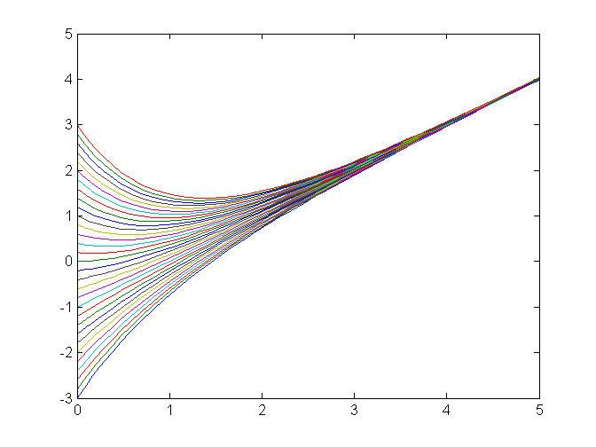
figure(figureforbis1)
hold on
plot(t, y)
title 'direction field and solution curves for dy/dt + y = t'
hold off

% Let's also note that if we solve the equation for y' and
% take the partial wrt to y, we get -1, which is < 0. So the
% equation is stable everywhere as the graphic suggests.
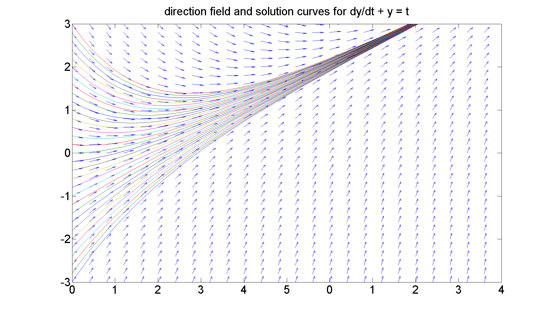
Now let's move on to the first of the two equations without symbolic solutions. We'll choose the parameters to match those that gave us the best direction field earlier in the session. Specifically, we'll restrict the t-axis to [0, 6] and the initial y-values to vary between 0.2 and 5, and we'll overlay the direction field.
% Here's the code:
g = @(t, y) -sqrt(y) + t;
figure(figureforbisonehalf)
[t, y] = ode45(g, [0 6], 0.2:0.2:5);
hold on
plot(t, y)
title 'direction field and solution curves for dy/dt + sqrt(y) = t'

% Again, if we solve for y' and take the partial wrt y, we
% obtain -(1/2)(1/sqrt(y), which for positive y,
% is again < 0, so we have stablity as the graphic suggests.
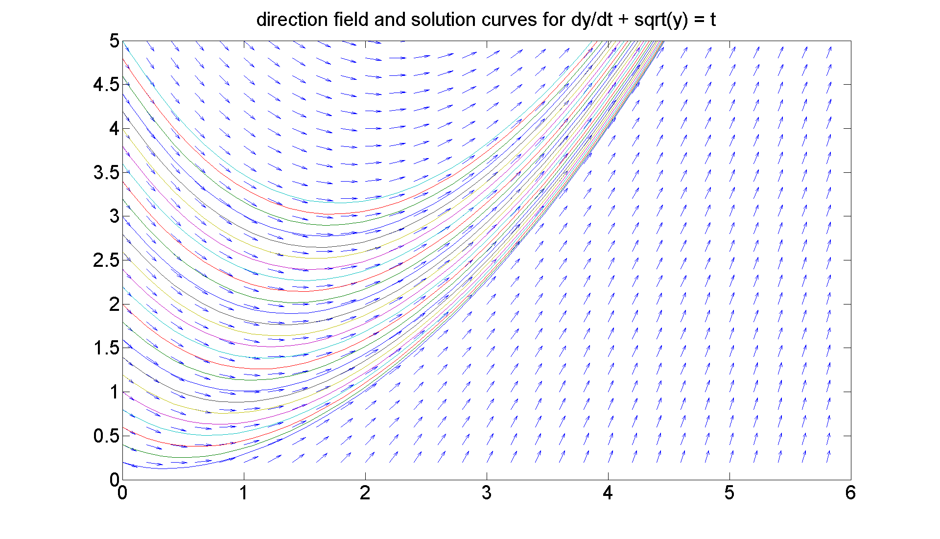
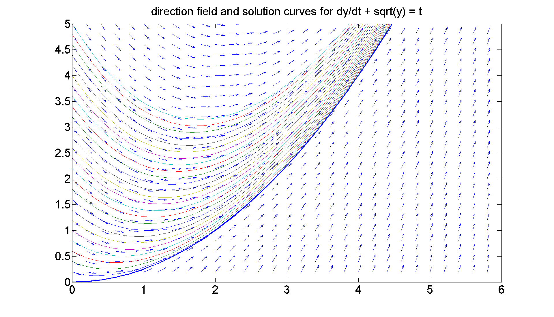
By the way, I suggested that the asymptotic curve for all the solutions was y = (1/4)t^2. Let's superimpose that curve on the graph.
Z = 0:0.2:5;
plot(Z, (1./4).*Z.^2, 'LineWidth', 2)
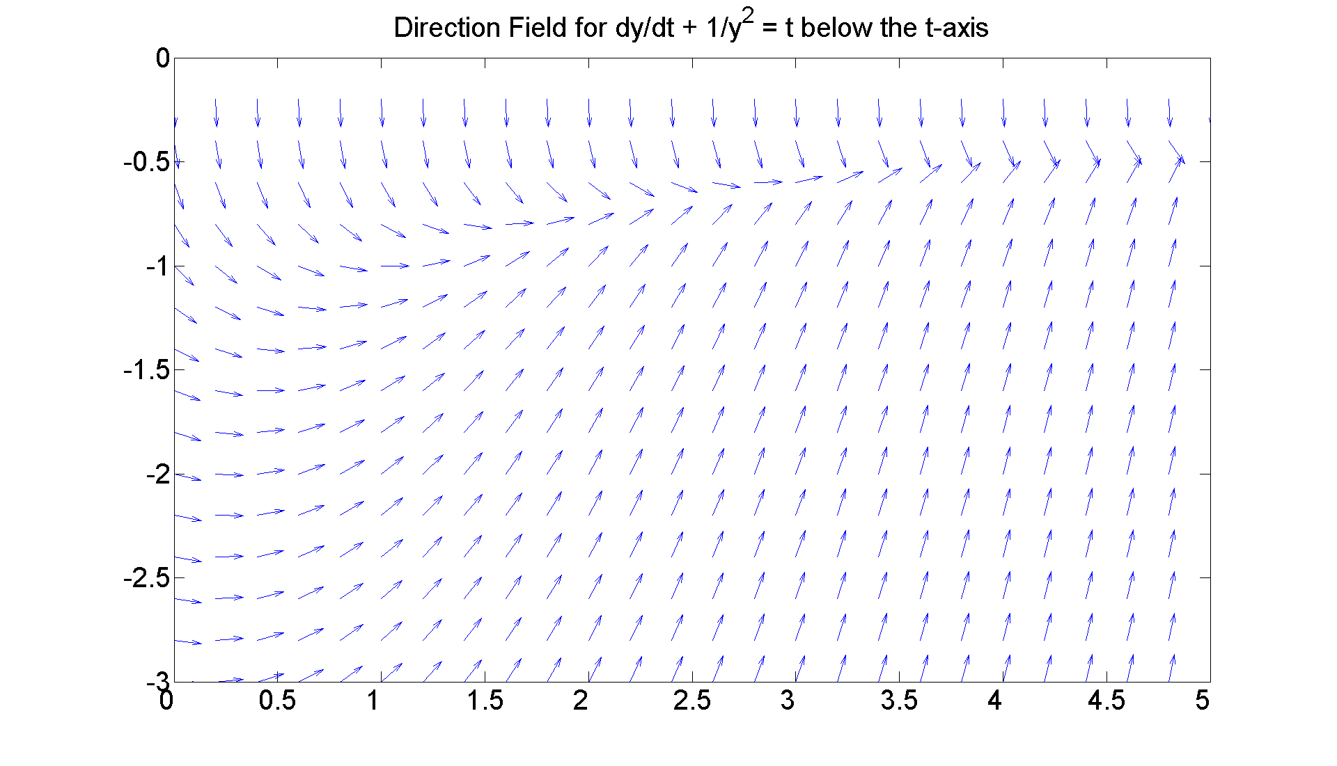
Finally, let's look at the most intractable case and see whether we can clear up the mystery that we encounted when we drew the direction field. Because of the term 1/y^2 in the differential equation, we know that there are problems on the t-axis. Let's break the problem into two domains, initial data above the t-axis and then below the t-axis. In each case, I'll first redraw the direction field, then plot some numerical solution curves and finally combine them. Before we do so, let's apply the partial wrt y test. It is 2y^(-3), which suggests stability below the t-axis and instability above. Let's handle the stable case first:
figure; set(gcf, 'Position', [1 1 1920 1420])
[T, Y] = meshgrid(0:0.2:5, -3:0.2:-0.2);
S = -1./Y.^2 + T;
L = sqrt(1 + S.^2);
quiver(T, Y, 1./L, S./L, 0.5), axis([0 5, -3 0])
title 'Direction Field for dy/dt + 1/y^2 = t below the t-axis'
set(get(gca, 'Title'),'Fontsize', 25)
set(gca,'XTickLabel',get(gca, 'XTickLabel'),'FontSize',25)
figureforbisminustwobottom = gcf

% Not so clear what is going on. Best guess is that solution
% curves that start far down on the y-axis tend toward the
% t-axis asymptotically; and those that start on the y-axis
% up near zero first decline and then move back up toward
% the t-axis asymptotically also. There also seem to be
% solution curves that come off the t-axis vertically down
% and then tend back toward it asymptotically,
% We'll verify some of this by first looking at
% a single curve, then a family and then by superimposing
% the direction field.
figureforbisminustwobottom =

     6
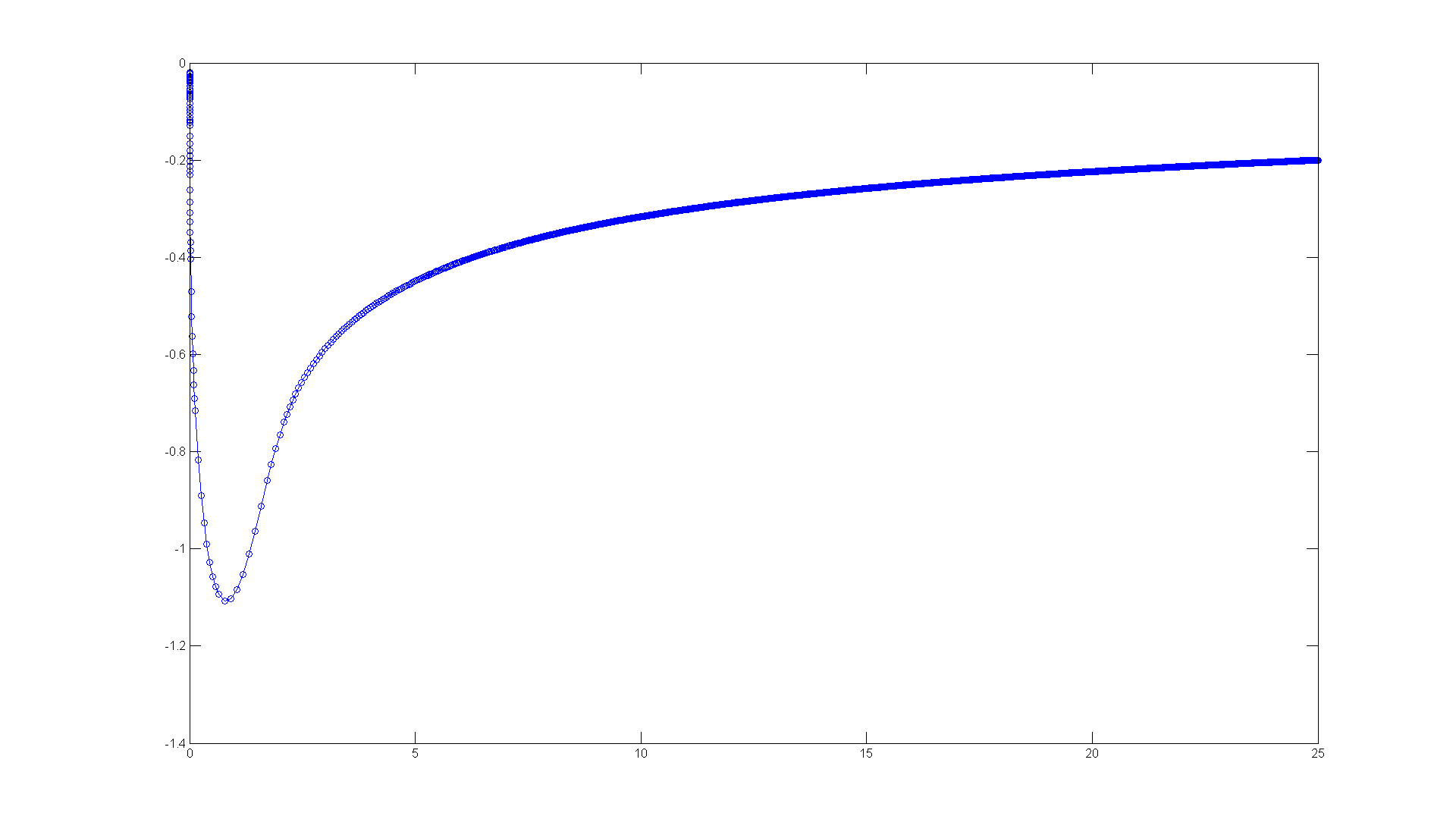
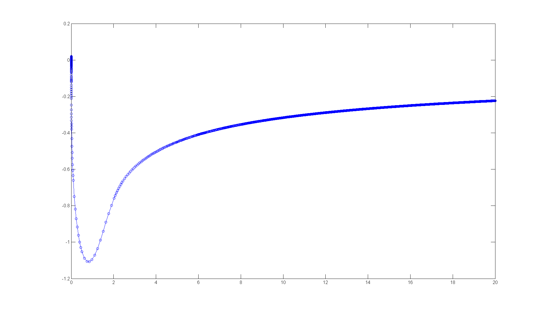
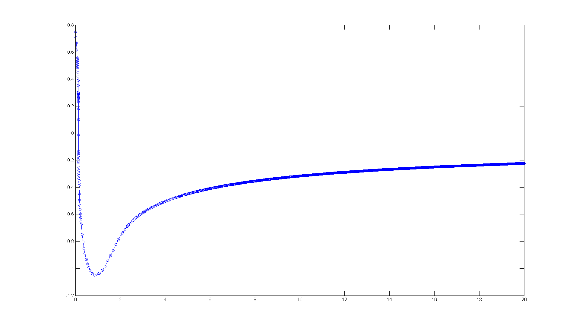
h = @(t, y) -1./y.^2 + t
figure; set(gcf, 'Position', [1 1 1920 1420])
ode45(h, [0 25], -0.02)

% The sharp turn is consisten with the
% direction field. But it's not clear that the asymptote
% is the t-axis. Can you explain from the differential
% equation why that must be so?
%           y' + 1/y^2 = t

% Now for more
% solution curves superimposed on the direction field.
h =

    @(t,y)-1./y.^2+t
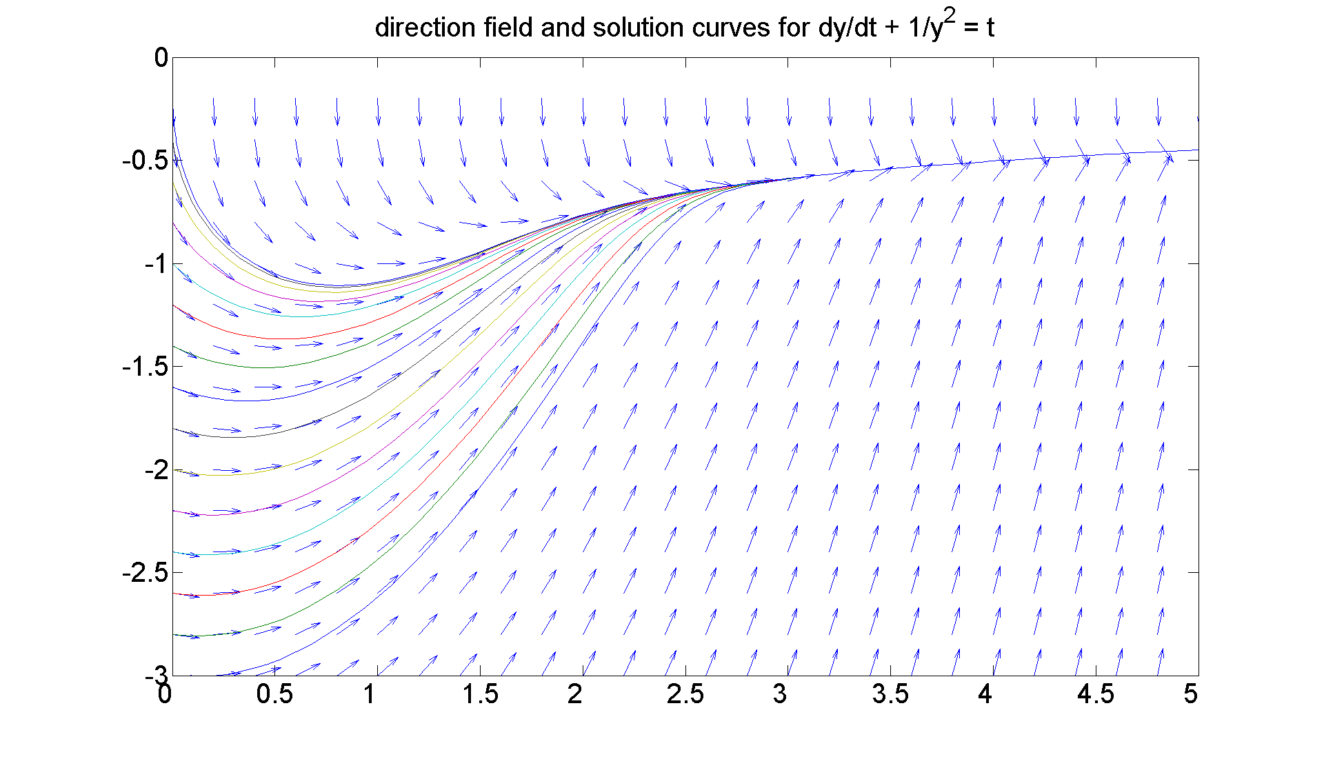
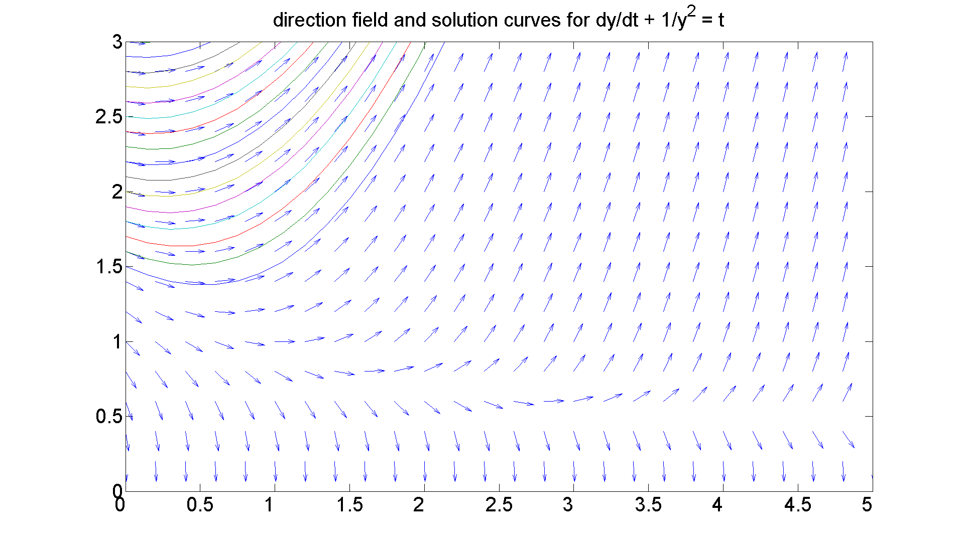
figure(figureforbisminustwobottom)
[t, y] = ode45(h, [0 6], -3:0.2:-0.2);
hold on
plot(t, y)
title 'direction field and solution curves for dy/dt + 1/y^2 = t'
hold off
Observations
I want to examine this picture a little more closely and make three observations:
% 1. The solution curves appear to be of two distinct types:
% those that start on the y-axis, perhpas decrease slightly for a
% bit and then increase slowly toward the t-axis; and those that
% seem to start on the t-axis, come off it vertically down, and
% then also increase slowly back to the t-axis. Moreover,
% there seems to be a solution curve
% that separates the two behaviors. This is very reminiscent of
% the idea of a "separatrix," which we shall study later in
% the course.

% 2. For the former of the two types, the domain of definition
% of the solution curve appears to be the positive t-axis. But
% for the latter type, the solution curve is defined on an interval
% of the form (alpha, infty), for some positive number alpha.
% Those curves come off the t-axis with infinite negative slope.

% Question: Why for large t must the separatrix in fact be
% asymptotic to
%       y = -1/sqrt(t)?

% Answer: Stare at the diff eqn:
%        y' + (1/y^2) = t.
% y' is tending to zero, so 1/y^2 is asymptotic to t for large t.

% 3. All the solution curves are coming together as t->infty;
% which is what we expect since below the t-axis, we know
% from the partial test, that we have stability.
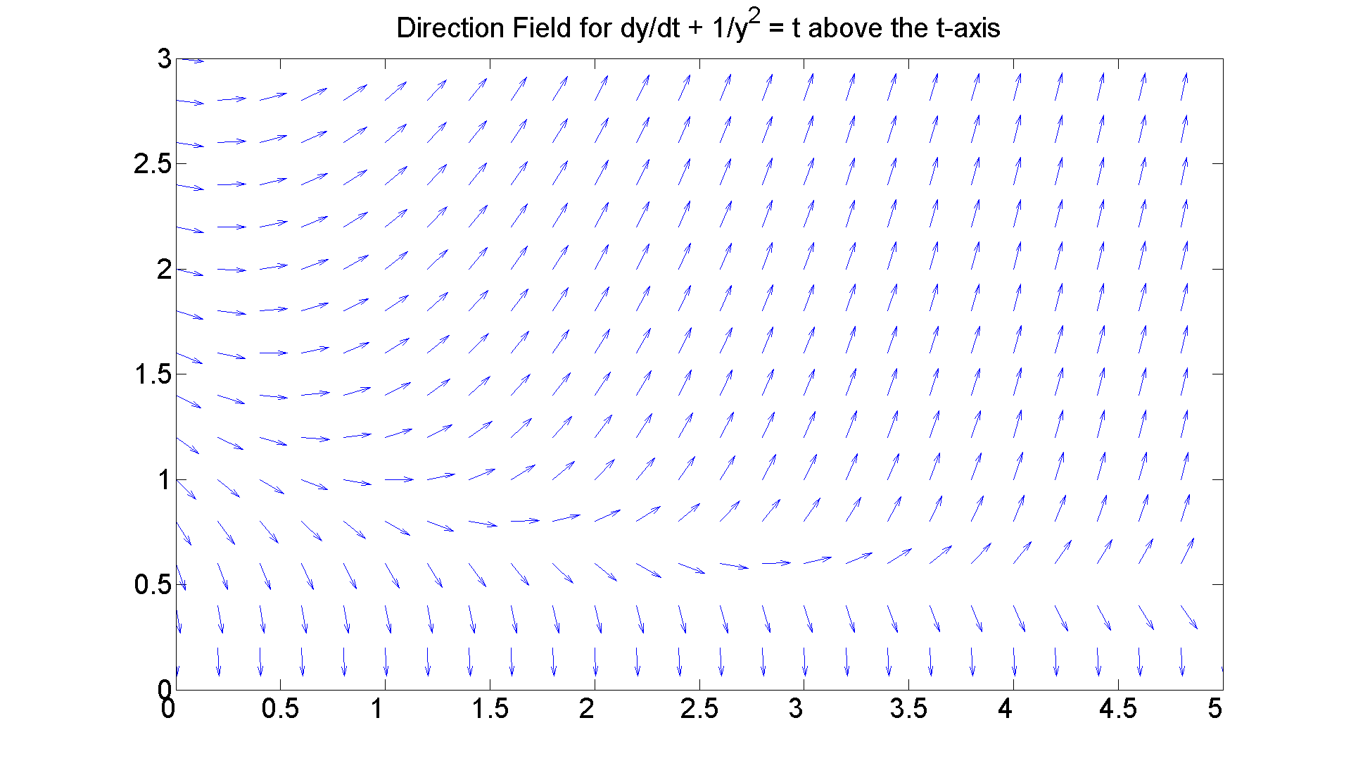
Our last chore is to examine the situation above the t-axis where the equation is unstable.
figure; set(gcf, 'Position', [1 1 1920 1420])
[T, Y] = meshgrid(0:0.2:5, 0.2:0.2:3);
S = -1./Y.^2 + T;
L = sqrt(1 + S.^2);
quiver(T, Y, 1./L, S./L, 0.5), axis([0 5, 0 3])
title 'Direction Field for dy/dt + 1/y^2 = t above the t-axis'
set(get(gca, 'Title'),'Fontsize', 25)
set(gca,'XTickLabel',get(gca, 'XTickLabel'),'FontSize',25)
figureforbisminustwotop = gcf

% Looks like the reverse of the previous situation where
% instead of the arrows coming together they are flying
% apart. Again, let's look at a typical problematic curve
% and then several curves.
figureforbisminustwotop =

     8
figure; set(gcf, 'Position', [1 1 1920 1420])
ode45(h, [0 20], 0.02)
You really see the instability there; the numerical solution jumped across the t-axis and started traveling on a solution curve below it. Here's an example where you can see it even better
figure; set(gcf, 'Position', [1 1 1920 1420])
ode45(h, [0 20], 0.75)
If we can stay far enough above the t-axis at our initial value, we can get a more reasonable graph.
figure(figureforbisminustwotop)
set(gcf, 'Position', [1 1 1920 1420])
[t, y] = ode45(h, [0 6], 1.5:0.1:3);
hold on
plot(t, y)
title 'direction field and solution curves for dy/dt + 1/y^2 = t'
Observations that are very similar to those above hold here:
% 1. Above a certain point the solution curves decrease slightly,
% then go flying off to infinity; but below that point, they crash
% into the t-axis. It's a little harder to see, but once again,
% there is a separatrix curve that separates the two behaviors.
% Reasoning as above, you should be able to see that for large t,
% that curve is asymptotic to
%       y = 1/sqrt(t).
In fact here is graphical evidence
W=0.2:0.1:5;
plot(W,1./sqrt(W),'LineWidth', 2)

2. The former solution curves are defined over the positive
t-axis, but the latter curves are defined on an interval of the form (0, beta), for some positive number beta.
% 3. The diagram illustrates the instability of the equation
% above the t-axis.
Final Thoughts
% Try to visualize the two portraits (above and below the t-axis)
% together. They fit together with vertical tangents to the
% solution curves at the t-axis. Try printing the two portraits and
% hold them up together.

% Exercise:
% See if you can figure out what the solution curves look like
% for negative t and try to do some analysis of the curves
% analogous to what I did here for positve t.