Contents

Transforms, especially the Laplace Transform

% In this lecture we shall study the concept of a transform
% and then specialize to the Laplace Transform. Suppose you
% have some collection of objects on which there are well
% defined operations. For example:

% **The set of all right triangles with various geometric
%       and algebraic operations; or

% **The set of Riemann Integrable functions on the
%       interval [-pi,pi] with various analytic operations; or

% **The set of piecewise continuous functions on the
%      positive x-axis with no more than exponential growth and
%      the operation of differentiation.

% You will recognize from the text (B&DiP, Ch 6) the last
% example as the set of functions for which we can take a
% Laplace Transform. We'll come back to that, but first
% let's consider the first two examples to get a
% feel for what a transform can do to help us solve concrete
% problems.

Right Triangles

% Given a right triangle, we shall associate with it a pair
% of real numbers in the set
%       {(x, y): 0 < x <= y}
% by assigning x to be the length of the shortest leg and
% y to be the length of the other leg.

% Now certain operations on the set of right triangles can
% be converted into operations on the pair of real numbers.
% For example, the operation of shrinking the size of each
% side of the triangle by the same amount, say lambda < 1,
% amounts to multiplying the coordinates (x, y) by lambda.
% Similarly with an expansion lambda > 1. One could also
% shrink or expand the two sides independently and that
% would correspond to multiplying the coordinates by
% distinct numbers. (One would have to restrict the
% multipliers to ensure that the multiple of x is less than
% the multiple of y.)

% Here is something more subtle. Given a
% right triangle, how do you obtain a new triangle in which
% the length of the shortest leg remains the same but the
% size of the angle between the shortest leg and the
% hypotenuse is three quarters its original size. How much
% shorter does the longer leg have to be? Well if theta is
% the angle in question, then first of all it needs to be
% greater than pi/4 radians in order for x to be the
% shorter side. And if it remains the shorter side in the new
% triangle, then (3/4)theta must also be greater than pi/4.
% So it must be that theta > pi/3. Now we multiply y
% by lambda. Then the geometric problem is transformed
% into the agebriac problem:

%       theta = arctan(y/x).
% Find lambda < 1 so that
%       (3/4) arctan(y/x) = arctan(lambda*y/x).

% Not an easy problem by hand, but easy for Matlab.
clear all
close all

To illustrate, suppose x = 1 and y = 3. Then

x = 1; y = 3; theta = atan(y/x)
lambda = x * tan((3/4)*theta)/y

% So you have to shorten the longer leg by a factor of 0.4533.
% in order to reduce the angle by 25%.

theta =

    1.2490


lambda =

    0.4533

Here's a harder problem. Find all the right triangles whose perimeter equals its area? After applying the transform, that is, converting the triangle into a pair of real numbers, the problem becomes: solve the equation (1/2)xy = x + y + sqrt(x^2 + y^2).

% That is some kind of quadratic curve.
% Let's see whether Matlab can simplify the equation
clear all
syms x y; simplify(((1/2)*x*y - (x+y))^2 - (x^2+y^2))

 
ans =
 
-(x*y*(4*x + 4*y - x*y - 8))/4
 

Since x and y are both non-zero, the equation further simplifies to 4*x + 4*y - x*y - 8 = 0.

% That is actually a hyperbola as you can see by making the
% substitution
% x = u + v, y = u - v.
syms u v; expr = 4*x + 4*y - x*y - 8; subs(expr, [x y], [u+v u-v])
expand(ans)

 
ans =
 
8*u - (u + v)*(u - v) - 8
 
 
ans =
 
- u^2 + 8*u + v^2 - 8
 

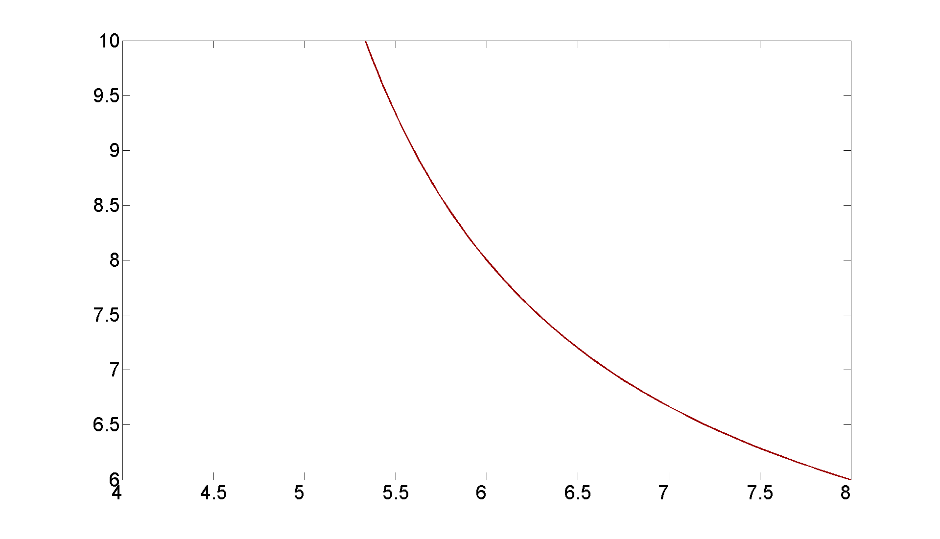
Also a little inspection reveals that x = 6, y = 8 is a point on the curve. So now we can draw it.

figure; set(gcf, 'Position', [1 1 1920 1420])
[X, Y] = meshgrid(4:0.1:8, 6:0.1:10);
contour(X, Y, (1./2).*X.*Y - (X + Y + sqrt(X.^2 + Y.^2)), [0 0],...
    'LineWidth',2,'Color',[.6 0 0])
set(gca,'XTickLabel',get(gca, 'XTickLabel'),'FontSize',25)

% See p. 28 in the HOLR book for an explanation of the
% option [0 0] in the contour command.

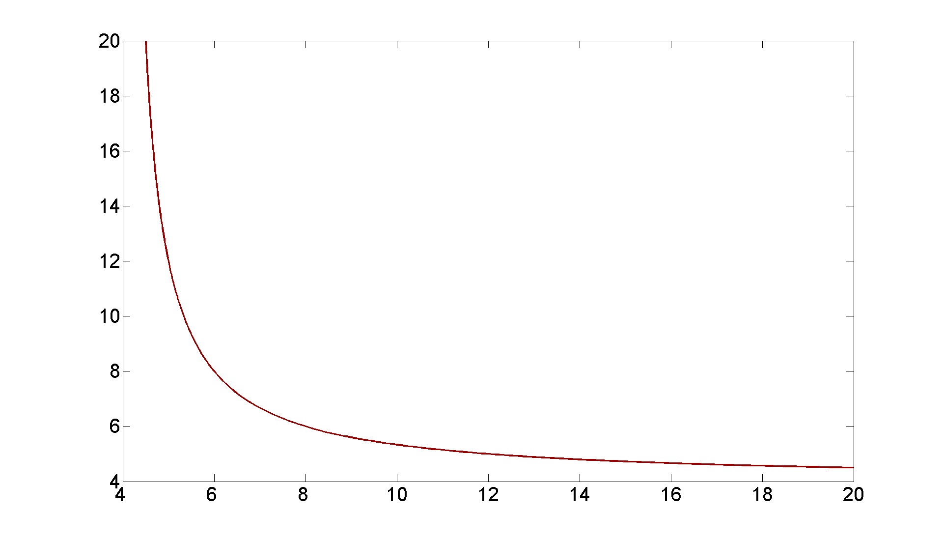
It's a very nice exercise to show algebraically that x = 4 is an asymptote of the hyperbola. It should be clear then that y = 4 is the other asymptote. Here is visual evidence:

figure; set(gcf, 'Position', [1 1 1920 1420])
[X, Y] = meshgrid(4:0.1:20, 4:0.1:20);
contour(X, Y, (1./2).*X.*Y - (X + Y + sqrt(X.^2 + Y.^2)), [0 0],...
    'LineWidth',2,'Color',[.6 0 0])
set(gca,'XTickLabel',get(gca, 'XTickLabel'),'FontSize',25)

Another nice exercise is to show that the only isosceles triangle which has equal perimeter and area corresponds to x = 4 + sqrt(8).

% Here is how to do it:
[a,b]=solve([x-y,expr])
% Why is only one answer legit?

 
a =
 
 2*2^(1/2) + 4
 4 - 2*2^(1/2)
 
 
b =
 
 2*2^(1/2) + 4
 4 - 2*2^(1/2)
 

Now for the second example.

% We consider the functions on [-pi, pi] that are Riemann
% integrable. You will have to look back at your calculus
% book if you don't remember upper sums and lower sums, etc.
% Certainly all continuous functions are
% integrable, but there are others, like
%       f(x) = 1/sqrt(|x|).
clear all
close all
syms x
figure; set(gcf, 'Position', [1 1 1920 1420])
ezplot(1/sqrt(x), [0 1])
set(get(gca, 'Title'),'Fontsize', 25)
set(gca,'XTickLabel',get(gca, 'XTickLabel'),'FontSize',25)

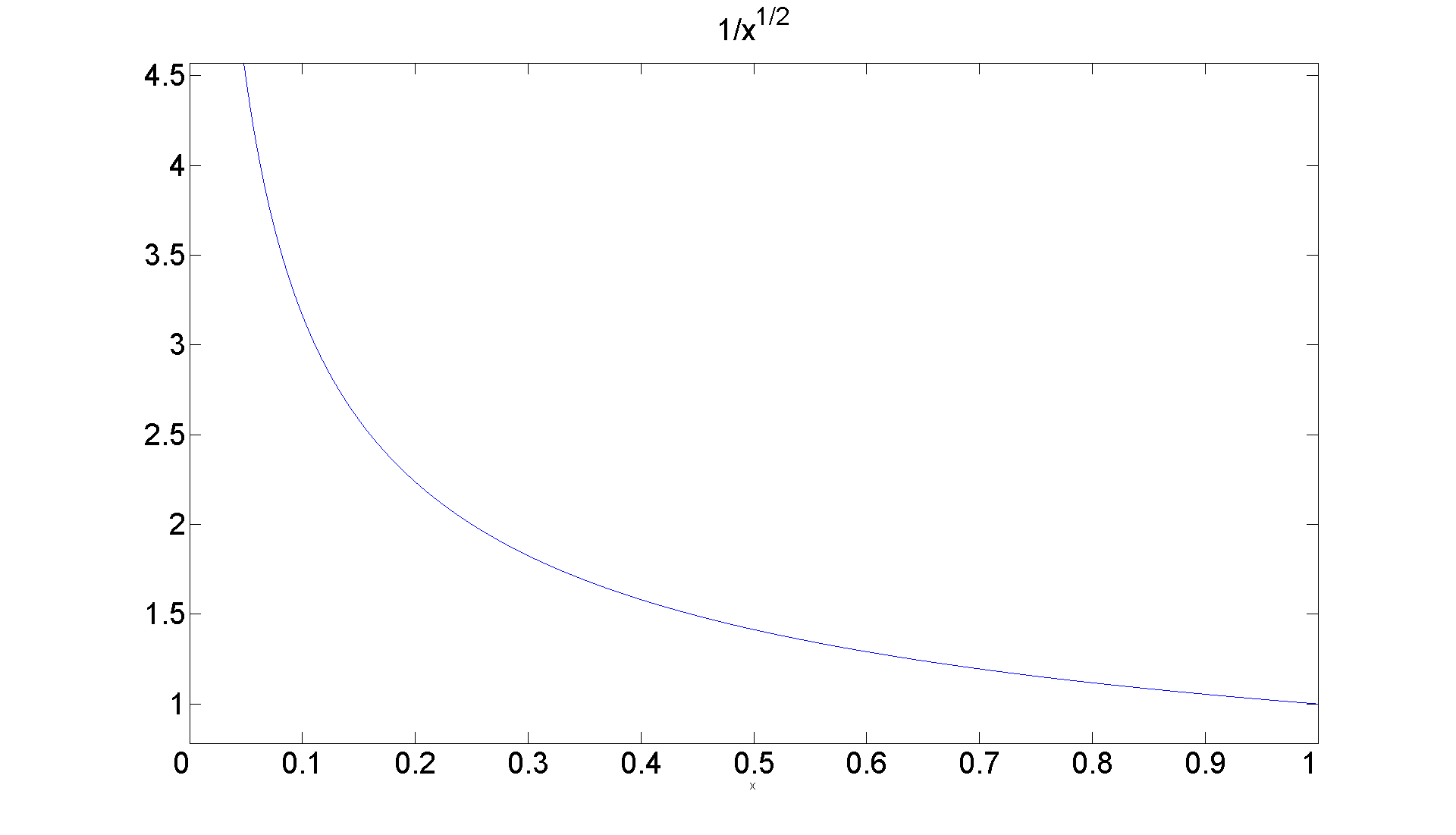
Clearly the y-axis is a vertical asymptote for the curve; Still, there is a finite area under the curve:

int(1/sqrt(x), 0, pi)

 
ans =
 
2*pi^(1/2)
 

Now for the transform. To every such function we associate or transform it to a sequence of complex numbers via the following formula:

% a_n = (1/2*pi)int_-pi^pi(e^(-i n t) f(t) dt, -inf < n < inf

% This transform is bound up with the theory of
% Fourier Series that you will certainly meet in later Math,
% Physics or Engineering courses. There are many interesting
% properties that relate the function f(t) to the
% sequence {a_n}, which comprises in fact the
% Fourier Coefficients of f.

% The associated Fourier Series is nothing more than
%       sum_{-inf}^{inf} a_n e^{i n t}.

% We can use this observation and the transform to solve the
% following problem. Which functions are square integrable?
% That is, when is it true that
%       int_-pi^pi |f(t)|^2 dt < inf.

% It's not true always as you can see from the example
%       f(t) = 1/sqrt(|t|).

 int(1/x, 0, pi)

 
ans =
 
Inf
 

We compute as follows _ int-pi^pi f(t)^2 dt = int_-pi^pi f(t)f(t) dt ________

%= int_-pi^pi [sum_{-inf}^{inf} a_n e^{i n t} sum_{-inf}^{inf} a_m e^{i m t}dt
%
% But (1/2pi)*int_-pi^pi e^{i j t}dt =0 unless j = 0,
% in which case it is 1.
%
%  So the above reduces to
%
%   sum_{-inf}^{inf} |a_n|^2.

% This solves the problem. An integrable function is
% square integrable precisely when its Fourier coefficients
% comprise a square summable sequence.

The Laplace Transform

Finally we look at the collection of functions that we have identified for which we can take a Laplace Transform, namely:

% The set of piecewise continuous functions on the positive
% x-axis with no more than exponential growth.
% The Laplace Transform of such a function f(t) is then
% defined as

%       L{f}(s) = F(s) = int_0^inf e^{-st} f(t) dt.

% The improper integral converges because of the assumptions
% on the growth of f. F(s) is a continuous function that
% decays to zero as s -> inf. The key property of the
% Laplace Transform that makes it useful in the study
% of differential equations is that it converts the operation
% of differentiation into mutiplication by the Laplace
% Transform variable; thus analytic problems in differential
% equations are converted into algebraic problems. The
% formulaic expression of the conversion is
% computed in the text as:

%   L{f'}(s) = s L(f}(s) - f(0)
%   L{f''}(s) = s^2 L{f}(s) - s f(0) - f'(0),

% perfect for initial value problems; and especially suited
% to problems involving discontinuous functions for which
% Laplace transforms can be computed.

A nice scheme for using Matlab to implement solutions via the Laplace Transform is presented in DEwM. Let's use it to solve the following explicit problem:

%       y''(t) + 2 y'(t) - 2 y(t) = g(t) + delta_2(t),
%       y(0) = 1, y'(0) = -1,

% where delta_2 is the Dirac generalized function
% concentrated at t = 2, and g(t) is given as follows:

% g(t) = 0, t < 0; t^2, 0<= t <1; 2, 1 <= t.

% Note that g is discontinuous at t = 1, but the full right side
% of the equation will also be discontinuous at t = 2, because
% of the Dirac delta function concentrated there.

clear all
close all

Here is the scheme presented in DEwM:

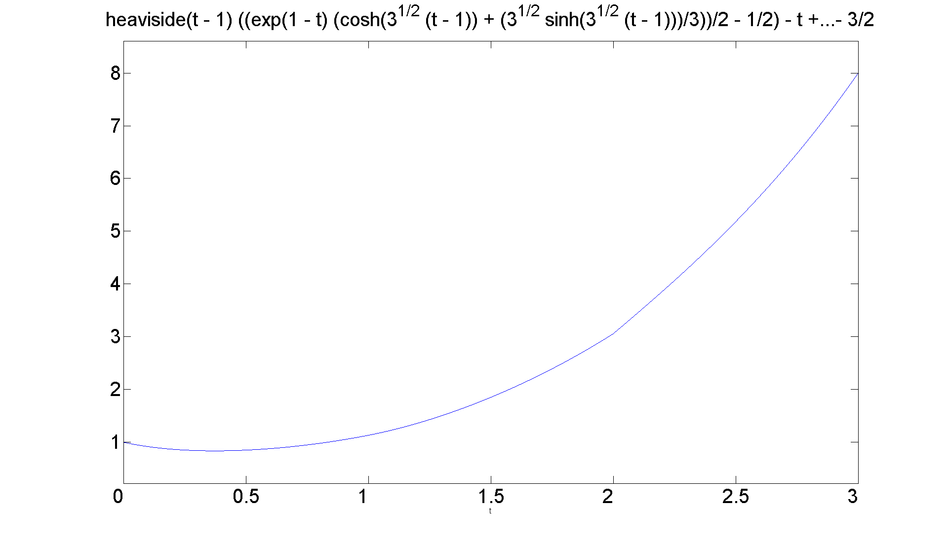
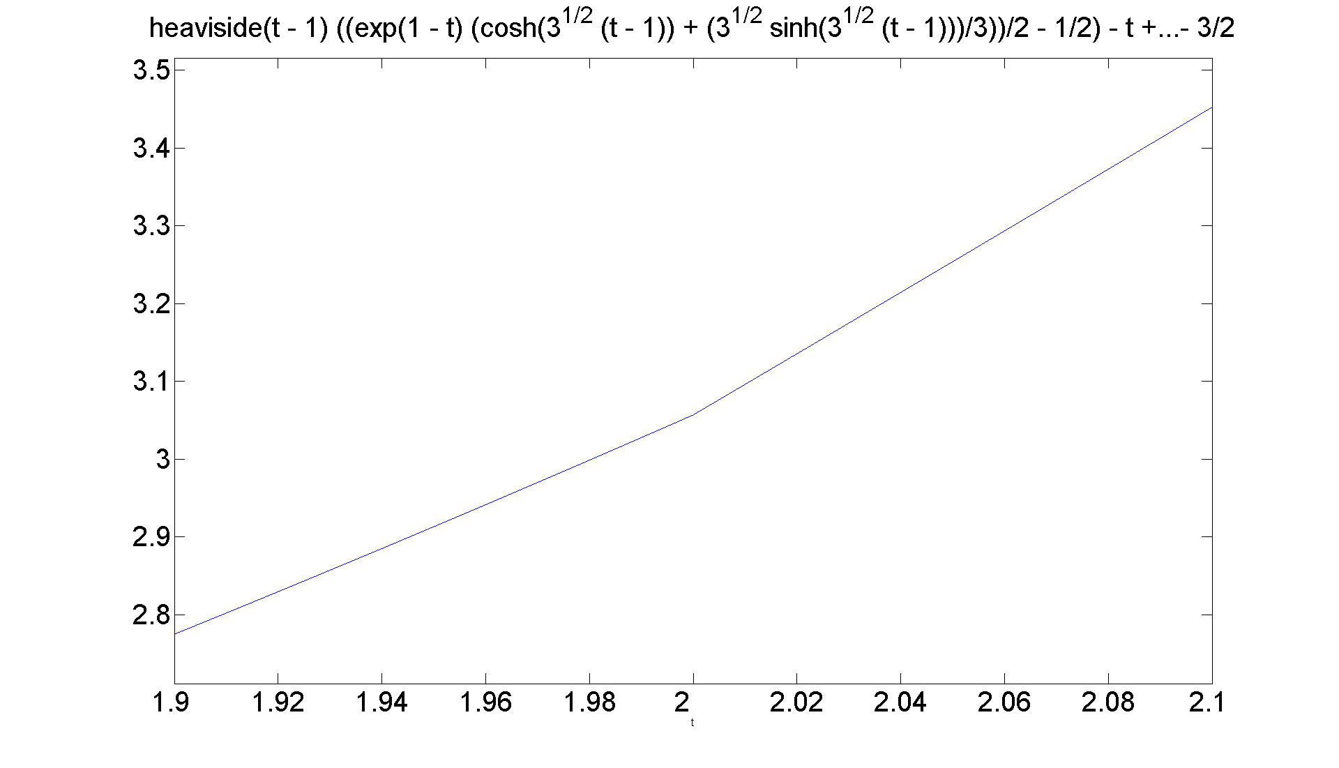
syms s t Y
g = ['heaviside(t)*t^2 + heaviside(t - 1)*(2 - t^2)'];
rhs = strcat(g,'+ dirac(t-2)');
eqn = sym(['D(D(y))(t) + 2*D(y)(t) - 2*y(t) = ' rhs]);
lteqn = laplace(eqn, t, s);
neweqn = subs(lteqn, {'laplace(y(t),t,s)', 'y(0)', 'D(y)(0)'}, {Y,1,-1});
ytrans = simplify(solve(neweqn,Y));
y = ilaplace(ytrans, s, t)
figure; set(gcf, 'Position', [1 1 1920 1420])
ezplot(y, [0 3])
set(get(gca, 'Title'),'Fontsize', 25)
set(gca,'XTickLabel',get(gca, 'XTickLabel'),'FontSize',25)

% Mention that the "simplify" command is missing in the book.
% Please use it when employing this template for solving eqns
% by the Laplace transform with Matlab.

% The graph illustrates a point made in DEwM. The solution
% function will be differentiable at t = 1, but only
% continuous at t = 2. That might be a little hard to see
% from the graph, so

 
y =
 
heaviside(t - 1)*((exp(1 - t)*(cosh(3^(1/2)*(t - 1)) + (3^(1/2)*sinh(3^(1/2)*(t - 1)))/3))/2 - 1/2) - t + 2*heaviside(t - 1)*(t/2 - (3*exp(1 - t)*(cosh(3^(1/2)*(t - 1)) + (5*3^(1/2)*sinh(3^(1/2)*(t - 1)))/9))/4 + (t - 1)^2/4 + 1/4) - t^2/2 + 2*heaviside(t - 1)*(t/2 - (exp(1 - t)*(cosh(3^(1/2)*(t - 1)) + (2*3^(1/2)*sinh(3^(1/2)*(t - 1)))/3))/2) + (cosh(3^(1/2)*t) - (3^(1/2)*sinh(3^(1/2)*t))/3)/exp(t) + (3*(cosh(3^(1/2)*t) + (5*3^(1/2)*sinh(3^(1/2)*t))/9))/(2*exp(t)) + (3^(1/2)*sinh(3^(1/2)*t))/(3*exp(t)) + (3^(1/2)*sinh(3^(1/2)*(t - 2))*heaviside(t - 2)*exp(2 - t))/3 - 3/2
 

figure; set(gcf, 'Position', [1 1 1920 1420])
ezplot(y, [1.9 2.1])
set(get(gca, 'Title'),'Fontsize', 25)
set(gca,'XTickLabel',get(gca, 'XTickLabel'),'FontSize',25)

Finally, the formula for the solution has been computed, although not displayed. Let's take a look.

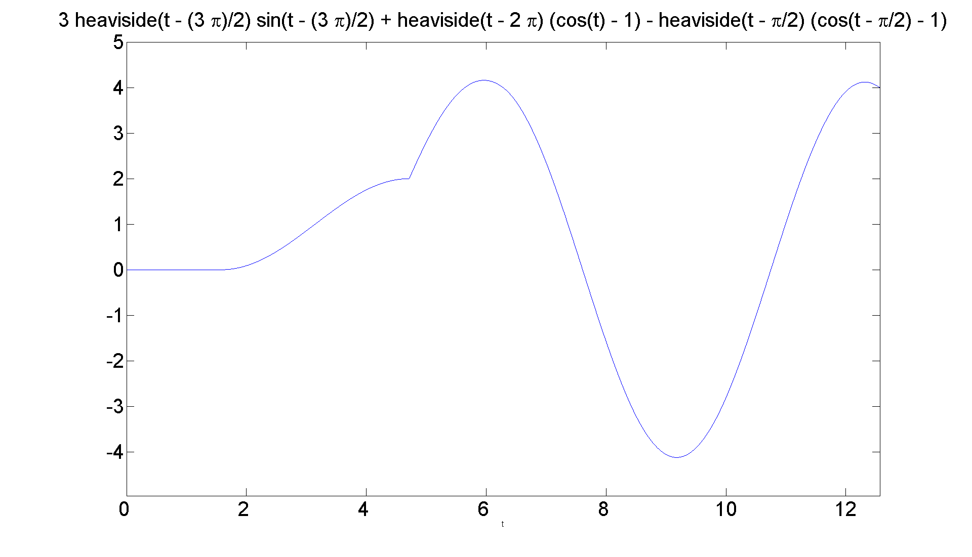
Another example: B&DiP, p. 343, #9. y''(t) + y(t) = u_pi/2(t) + 3*delta_3*pi/2(t) - u_2*pi(t), y(0) = 0, y'(0) = 0.

syms s t Y
g = ['heaviside(t-pi/2) - heaviside(t - 2*pi)'];
rhs = strcat(g,'+ 3*dirac(t-3*pi/2)');
eqn = sym(['D(D(y))(t) + y(t) = ' rhs]);
lteqn = laplace(eqn, t, s);
neweqn = subs(lteqn, {'laplace(y(t),t,s)', 'y(0)', 'D(y)(0)'}, {Y,0,0});
ytrans = simplify(solve(neweqn,Y));
y = ilaplace(ytrans, s, t)
figure; set(gcf, 'Position', [1 1 1920 1420])
ezplot(y, [0 4*pi])
set(get(gca, 'Title'),'Fontsize', 25)
set(gca,'XTickLabel',get(gca, 'XTickLabel'),'FontSize',25)

% Again, let's look at the solution formula.

 
y =
 
3*heaviside(t - (3*pi)/2)*sin(t - (3*pi)/2) + heaviside(t - 2*pi)*(cos(t) - 1) - heaviside(t - pi/2)*(cos(t - pi/2) - 1)
 

Published with MATLAB® 7.13