Presentation5Spring12

Non-Linear Systems
Vector Fields
Linearized Analysis
Second Example -- a damped pendulum.
Phase Portraits
For example:
And then:

Non-Linear Systems

% In this presentation we will look at 2x2 systems of linear
% and non-linear 1st order, ordinary differential equations:

%       x' = f(x, y, t)
%       y' = g(x, y, t).

% These arise naturally in two ways: either from a single
% second order equation or from a problem that involves two
% dependent variables but only a single independent variable.
% The rotating rigid pendulum problem is an example of the
% former; and both the competing species and predator-prey
% problems are examples of the latter.

% For the pendulum, the second order equation is:

% theta''+lambda*theta'+(g/L)*sin(theta)=F(theta, theta', t),

% where lambda is a damping coefficient, g is the
% gravitational constant, L is the length of the pendulum
% and F is an impressed external force that may depend on
% position, velocity and time. If we set

%       x = theta, y = theta'
% then we get the system

%       x' = y
%       y' = -lambda*y -(g/L)*sin x + F(x, y, t).

% For the purposes of this lecture, I shall only consider
% autonomous systems, i.e., those in which time, i.e., t,
% is not present on the right side of the equations; thus

%       x' = f(x, y)
%       y' = g(x, y).

% Both the competing species and the predator-prey models,
% as well as the rotating pendulum (with no external force),
% fall into this category.

% What is a solution to such a system. It is a pair of
% functions

%       x = phi(t), y = psi(t)
% defined on some interval t_1 < t < t_2, that satisfy

%       phi'(t) = f(phi(t), psi(t))
%       psi'(t) = g(phi(t), psi(t)),

% on the interval. But such a pair of functions can be
% thought of as parametric equations for a curve in the
% x-y plane. Moreover, it follows from the uniqueness
% theorem, that if two solutions of the same autonomous
% system intersect, then they must be identical curves--
% that is, the two solutions are (possibly different
% parameterizations of) the same curve.

% We say that the system is linear if f and g are linear
% functions of x  and y, that is

%       x' = ax + by
%       y' = cx + dy.

% In the text and in the HOLR book, it is shown, using the easily
% computed eigenvalues and eigenvectors of the matrix
%       [a, b; c, d]
% how to write down explicit solution formulas for a
% linear system.

% On the other hand, if a system is non-linear, generally it
% is impossible to find formula solutions. Instead we pursue
% three distinct methods for analyzing non-linear systems:
%       1. Vector Fields -- a geometric method
%       2. Linearized Analysis -- an algebraic method
%       3. A numerically-generated Phase Portrait -- an
%           analytic method.

% Let's look at some examples to illustrate the three
% methods.

Vector Fields

% A simple linear problem:
% Consider the system
%       x' = -x + 2*y
%       y' = -3*x - y.

% Here is the corresponding vector field:
clear all
close all
figure; set(gcf, 'Position', [1 1 1920 1120])
[X, Y] = meshgrid(-3:0.2:3, -3:0.2:3);
U = -X + 2.*Y;
V = -3.*X - Y;
L = sqrt(U.^2 + V.^2);
quiver(X, Y, U./L, V./L, 0.4, 'LineWidth', 2)
axis equal tight
xlabel ('x', 'FontSize',25)
ylabel ('y', 'FontSize',25)
title ('Vector Field for a Linear Sysytem', 'FontSize',25)
set(gca,'XTickLabel',get(gca, 'XTickLabel'),'FontSize',25)

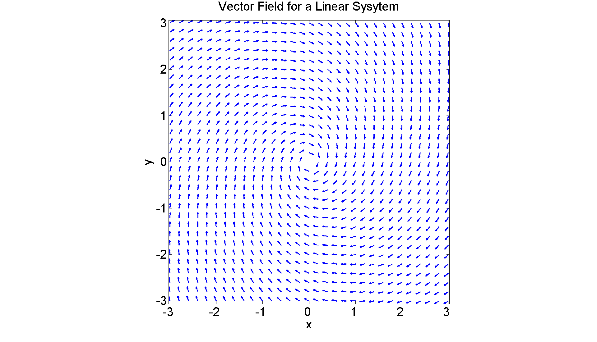
It should be clear that this is a case in which the origin is an asymptotically stable spiral point. (The direction of motion is indicated by the arrowheads.) Let's just check that by finding the eigenvalues of the coefficient matrix:

A = [-1, 2; -3, -1];
[xi, R] = eig(sym(A))

% Confirmed: complex conjugate eigenvalues with negative
% real part.

 
xi =
 
[ (6^(1/2)*i)/3, -(6^(1/2)*i)/3]
[             1,              1]
 
 
R =
 
[ - 6^(1/2)*i - 1,             0]
[               0, 6^(1/2)*i - 1]

Now let's compute a vector field for a non-linear problem. I'll do the undamped pendulum. (Here, and below, I'll take L = g for simplicity.)

%       x' = y
%       y' = -sin(x)

figure; set(gcf, 'Position', [1 1 1920 1420])
[X, Y] = meshgrid(-2:0.2:8, -2:0.2:2);
U = Y;
V = -sin(X);
L = sqrt(U.^2 + V.^2);
quiver(X, Y, U./L, V./L, 0.4, 'LineWidth', 2)
axis equal tight
xlabel ('x', 'FontSize',25)
ylabel ('y', 'FontSize',25)
title ('Vector Field for the undamped pendulum', 'FontSize',25)
set(gca,'XTickLabel',get(gca, 'XTickLabel'),'FontSize',25)

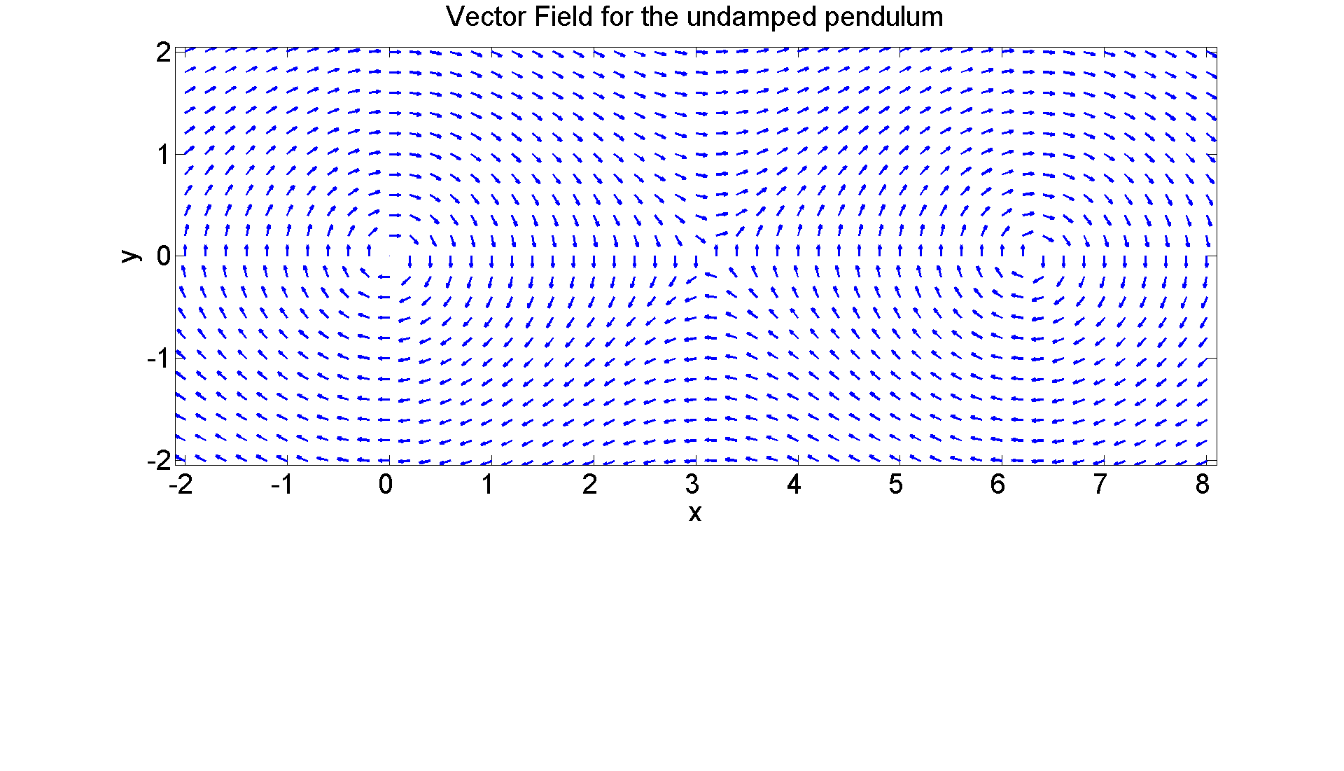
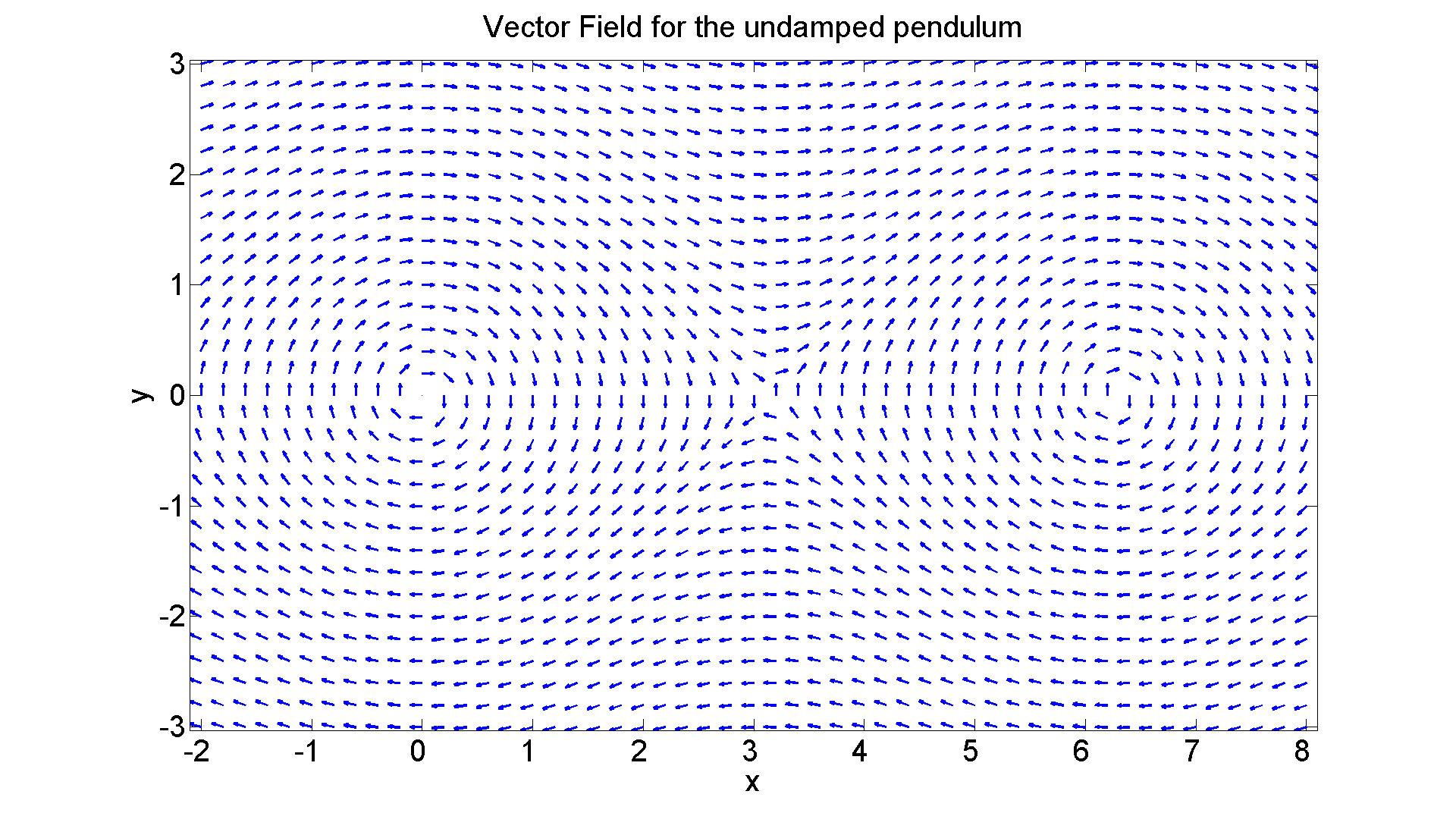
The only equilibrium points are (n*pi,0). If you leave the pendulum with no initial displacement and no initial velocity, nothing happens. If you move it to the right a little and release, it swings back to the equilibrium position, goes through it to the same extent on the other side and then oscillates back and forth forever. If you move it to the upwards vertical, it remains precariously perched there. If you move it past the vertical and release, it oscillates (around the point (2pi,0)) forever. If you don't move it to start, but instead hit it, it will oscillate as before--provided you don't hit it too hard. If you hit it too hard, it will oscillate round and round forever. How hard is too hard? Let's redo the picture allowing for a bigger initial velocity.

figure; set(gcf, 'Position', [1 1 1920 1120])
[X, Y] = meshgrid(-2:0.2:8, -3:0.2:3);
U = Y;
V = -sin(X);
L = sqrt(U.^2 + V.^2);
quiver(X, Y, U./L, V./L, 0.4, 'LineWidth', 2)
axis equal tight
xlabel ('x', 'FontSize',25)
ylabel ('y', 'FontSize',25)
title ('Vector Field for the undamped pendulum', 'FontSize',25)
set(gca,'XTickLabel',get(gca, 'XTickLabel'),'FontSize',25)

% The critical value is apparently somewhere between 1 and 2;
% It's a nice exercise using ode45 (as we will momentarily
% when we draw phase portraits) to approximate the value.

Vector Field for a Peaceful Coexistence Competing Species Model x' = x(2 - 3x -y) y' = y(1 - x - y).

figure; set(gcf, 'Position', [1 1 1920 1120])
[X, Y] = meshgrid(0:0.1:2, 0:0.1:2);
U = X.*(2 - 3.*X - Y);
V = Y.*(1 - X - Y);
L = sqrt(U.^2 + V.^2);
quiver(X, Y, U./L, V./L, 0.3, 'LineWidth', 2)
axis tight
xlabel ('x', 'FontSize',25)
ylabel ('y', 'FontSize',25)
title ('Vector Field for Peaceful Coexistence Competing Species Model', 'FontSize',25)
set(gca,'XTickLabel',get(gca, 'XTickLabel'),'FontSize',25)

% Notice I refined the quiver parameters (as I did in some of the
% above graphs) a little to improve the picture. But it's a little
% hard to read from the graph what the exact equilibrium
% points are. So let's have Matlab compute them for us.

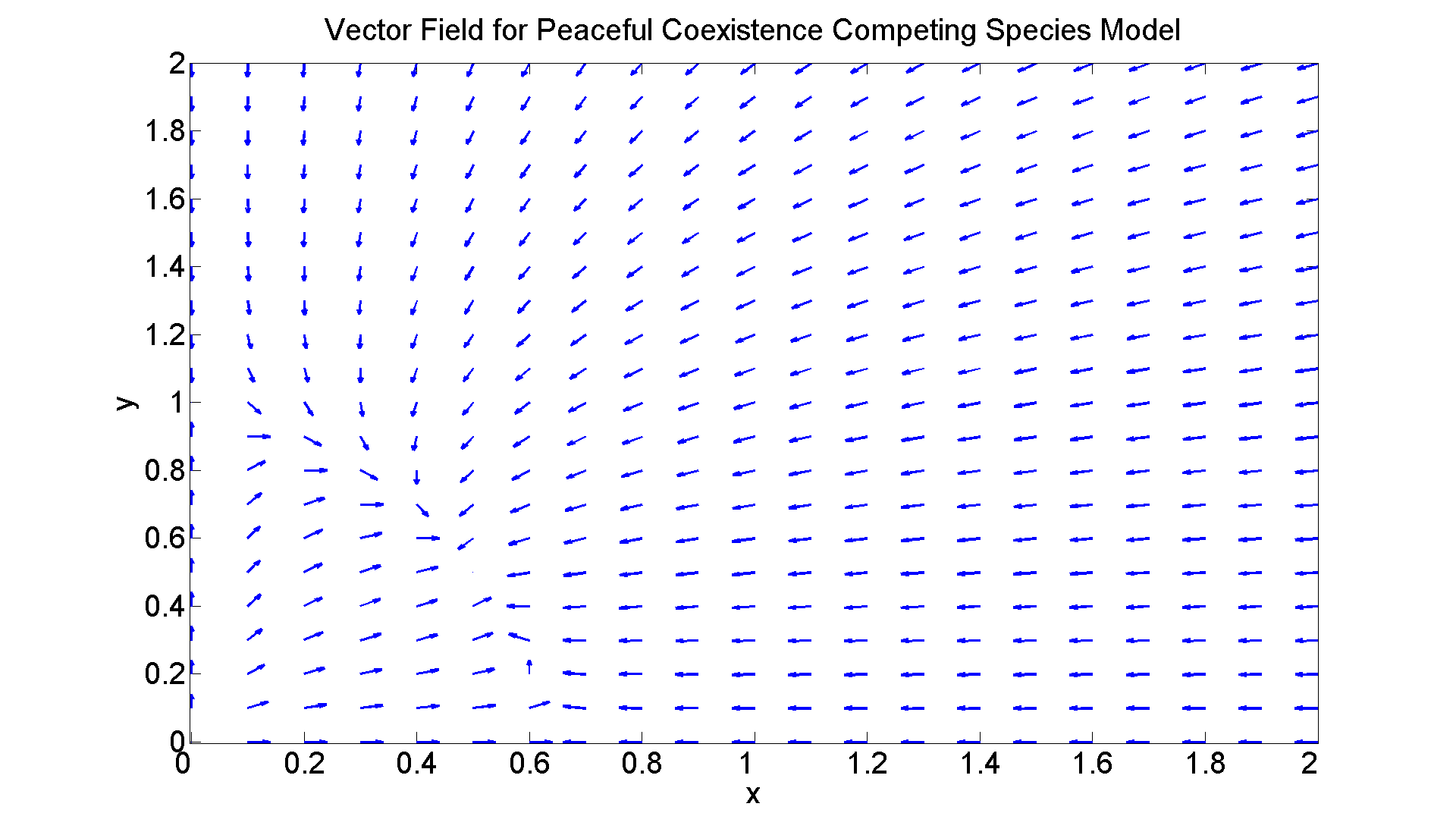
syms x y;
[a b]=solve([x*(2-3*x-y) y*(1-x-y)]);
disp('Critical points:'); disp([a b])

% They are: (0,0), (0,1), (2/3,0) and (1/2,1/2).

Critical points:
[   0,   0]
[   0,   1]
[ 2/3,   0]
[ 1/2, 1/2]

Linearized Analysis

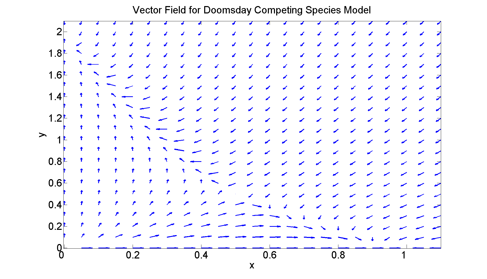
We'll do two examples here: the doomsday competing species model and a damped pendulum. First, the doomsday model x' = x(1 - x - y) y' = y(2 - 3x - y).

% There are four critical points: (0,0), (1,0), (0,2) and
% (1/2,1/2).
% Let's verify that:
syms x y
sys1 = x*(1 - x - y);
sys2 = y*(2 - 3*x - y);
[xc, yc] = solve(sys1, sys2, x, y); disp('Critical points:'); disp([xc yc])

Critical points:
[   0,   0]
[   0,   2]
[   1,   0]
[ 1/2, 1/2]

That corroborates the location of the critical points. I'll do the linearized analysis at just the last point:

A = jacobian([sys1 sys2], [x y])
evals = eig(A)
disp('Eigenvalues at (1/2,1/2):'); disp(double(subs(evals, {x, y}, {1/2, 1/2})))
% The saddle point at (1/2,1/2) is confirmed.

 
A =
 
[ 1 - y - 2*x,            -x]
[        -3*y, 2 - 2*y - 3*x]
 
 
evals =
 
 3/2 - (3*y)/2 - (x^2 + 14*x*y - 2*x + y^2 - 2*y + 1)^(1/2)/2 - (5*x)/2
 (x^2 + 14*x*y - 2*x + y^2 - 2*y + 1)^(1/2)/2 - (3*y)/2 - (5*x)/2 + 3/2
 
Eigenvalues at (1/2,1/2):
   -1.3660
    0.3660

Let's also look at the vector field for this Doomsday Competing Species Model

figure; set(gcf, 'Position', [1 1 1920 1120])
[X, Y] = meshgrid(0:0.05:1.1, 0:0.1:2.1);
U = X.*(1.0 - X - Y);
V = Y.*(2.0 - 3.*X - Y);
L = sqrt(U.^2 + V.^2);
quiver(X, Y, U./L, V./L, 0.3, 'LineWidth', 2)
axis tight
xlabel ('x', 'FontSize',25)
ylabel ('y', 'FontSize',25)
title ('Vector Field for Doomsday Competing Species Model', 'FontSize',25)
set(gca,'XTickLabel',get(gca, 'XTickLabel'),'FontSize',25)

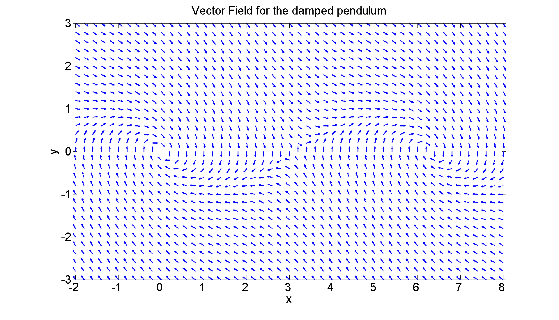
Second Example -- a damped pendulum.

We'll take the damping coefficient to be 1, so the system is x' = y y' = -sin(x) - y.

% The critical points are clearly the same as in the
% undamped problem, namely, (n*pi,0). When the pendulum was
% undamped, these points were stable circular points when n
% was even and unstable saddle points when n was odd. This
% time, the equilibrium points corresponding to odd n
% continue to be unstable saddle points, but when n is even,
% they become asymptotically stable spiral points as we can
% see by the following computation:

sys3 =  y;
sys4 = -y - sin(x);
A = jacobian([sys3 sys4], [x y])
evals = eig(A)

disp('Eigenvalues at (0,0):'); disp(double(subs(evals, {x, y}, {0, 0})))
disp('Eigenvalues at (pi,0):'); disp(double(subs(evals, {x, y}, {pi, 0})))

 
A =
 
[       0,  1]
[ -cos(x), -1]
 
 
evals =
 
 - (1 - 4*cos(x))^(1/2)/2 - 1/2
   (1 - 4*cos(x))^(1/2)/2 - 1/2
 
Eigenvalues at (0,0):
  -0.5000 - 0.8660i
  -0.5000 + 0.8660i

Eigenvalues at (pi,0):
   -1.6180
    0.6180

Once again, let's look at the vector field.

figure; set(gcf, 'Position', [1 1 1920 1120])
[X, Y] = meshgrid(-2:0.2:8, -3:0.2:3);
U = Y;
V = -sin(X) - Y;
L = sqrt(U.^2 + V.^2);
quiver(X, Y, U./L, V./L, 0.4, 'LineWidth', 2)
axis equal tight
xlabel ('x', 'FontSize',25)
ylabel ('y', 'FontSize',25)
title ('Vector Field for the damped pendulum', 'FontSize',25)
set(gca,'XTickLabel',get(gca, 'XTickLabel'),'FontSize',25)

Phase Portraits

Now we turn to the third method of analyzing non-linear systems, phase portraits generated by numerical solutions. We will look at three examples, and also reexamine the undamped pendulum that we studied previously using only its vector field. The three examples will all be predator-prey models.

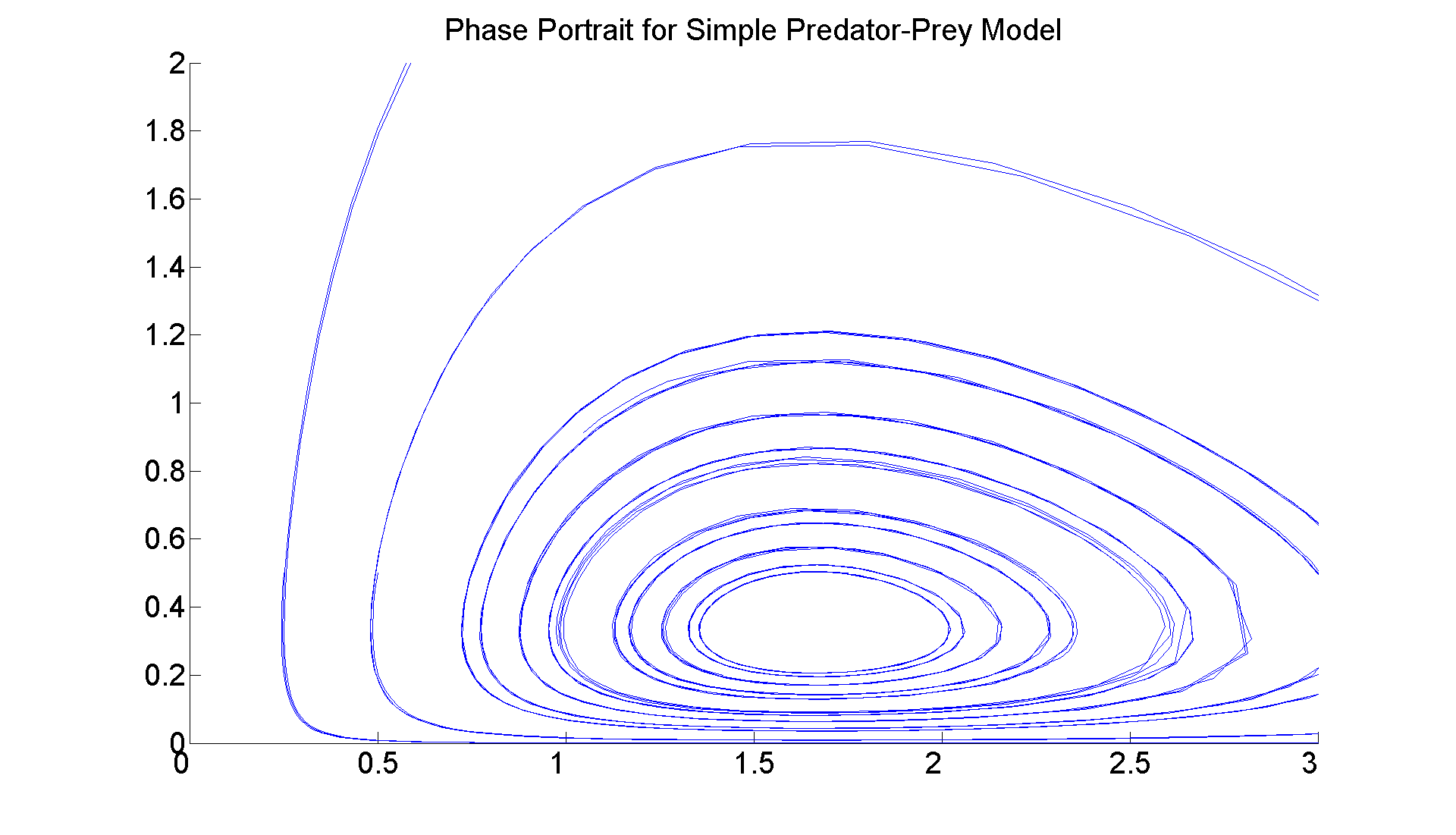
First example: x' = x*(1 - 3*y) y' = y*(3*x - 5).

% In PSF Problem 4 in Ran's sections, you are
% asked to both do the linearized analysis and produce a
% vector field for a very similar problem.
% Here we only generate a phase portrait.

figure; set(gcf, 'Position', [1 1 1920 1420])
hold on
f = @(t, x) [x(1)*(1 - 3*x(2)); x(2)*(3*x(1) - 5)];
for a = 0:0.25:3
	[t, xa] = ode45(f, [0 10], [a, 1/2]);
	plot(xa(:,1),xa(:,2))
end
axis([0 3 0 2])
title ('Phase Portrait for Simple Predator-Prey Model', 'FontSize',25)
set(gca,'XTickLabel',get(gca, 'XTickLabel'),'FontSize',25)

% This plot strongly suggests that the equilibrium position
% at approx (5/3,1/3) is stable. This is a standard
% predator-prey model that yields the origin as an unstable
% saddle point and the single stable interior point with
% stable populations. It is clear from the equations that
% indeed that point is (5/3,1/3). (Recall that the
% linearized analysis for this type of example does not give
% a conclusive answer as to the stability of the interior
% critical point. But the phase portrait -- and the vector
% field if you draw it--are pretty convincing.)

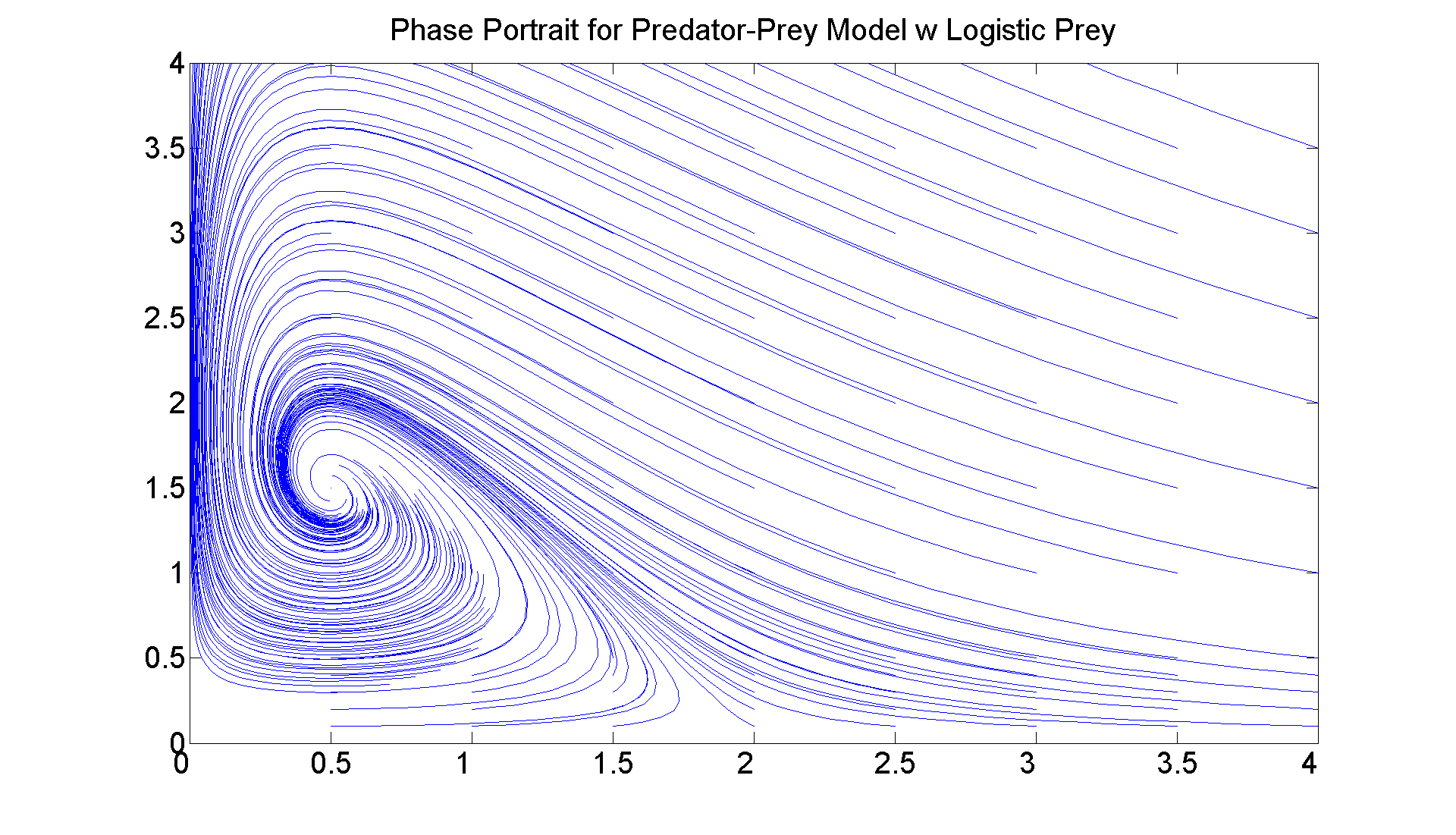
In the second example we modify the equations so that the prey, if left alone, satisfies a logistic equation-- very similar to PSF Problem 4 in Adam's sections: x' = x*(1 - x/2 - y/2) y' = y*(x/2 - 1/4).

figure; set(gcf, 'Position', [1 1 1920 1420])
f = @(t, x) [x(1)*(1 - x(1)/2 - x(2)/2); x(2)*(-1/4 + x(1)/2)];
for a = 0:0.5:4
   for b = [0 0.1 0.2 0.3 0.4 0.5 1 1.5 2 2.5 3 3.5 4]
      [t, xa] = ode45(f, [0 15], [a b]);
      plot(xa(:,1), xa(:,2))
      hold on
      %[t, xa] = ode45(f, [0 -5], [a b]);
      plot(xa(:,1), xa(:,2))
   end
end
axis([0 4 0 4])
title ('Phase Portrait for Predator-Prey Model w Logistic Prey', 'FontSize', 25)
set(gca,'XTickLabel',get(gca, 'XTickLabel'),'FontSize',25)

% This time the interior critical point, which from the
% equations (and the portrait) is clearly at (1/2, 3/2),
% is an asymptotically stable spiral point. There
% are two saddle points: (0,0) and (2,0). Note: I played
% around with the choice of initial data to maximize the
% quality of the graph.

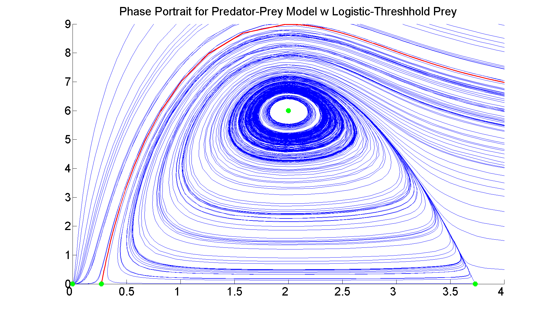
Finally, here is an example in which the prey satisfies a logistic-threshhold equation. You should recognize it since it is almost identical to PSF Problem 5 in all the sections: x' = x*(-1 + 4*x - y/2 - x^2) y' = y*(x - 2).

warning off all
f = @(t, x) [x(1)*(-1 + 4.*x(1) - 0.5.*x(2) - x(1)^2); x(2)*(x(1) - 2)];
figure; set(gcf, 'Position', [1 1 1920 1420])
axes; hold on
for a = 0.5:0.5:4
	for b = 0.5:9
		[t, xa] =ode45(f, [0 20], [a, b]);
		plot(xa(:,1),xa(:,2))
		[t, xa] = ode45(f, [0 -10], [a, b]);
		plot(xa(:,1),xa(:,2))
	end
end
axis([0 4 0 9])
title ('Phase Portrait for Predator-Prey Model w Logistic-Threshhold Prey', 'FontSize', 25)
set(gca,'XTickLabel',get(gca, 'XTickLabel'),'FontSize',25)

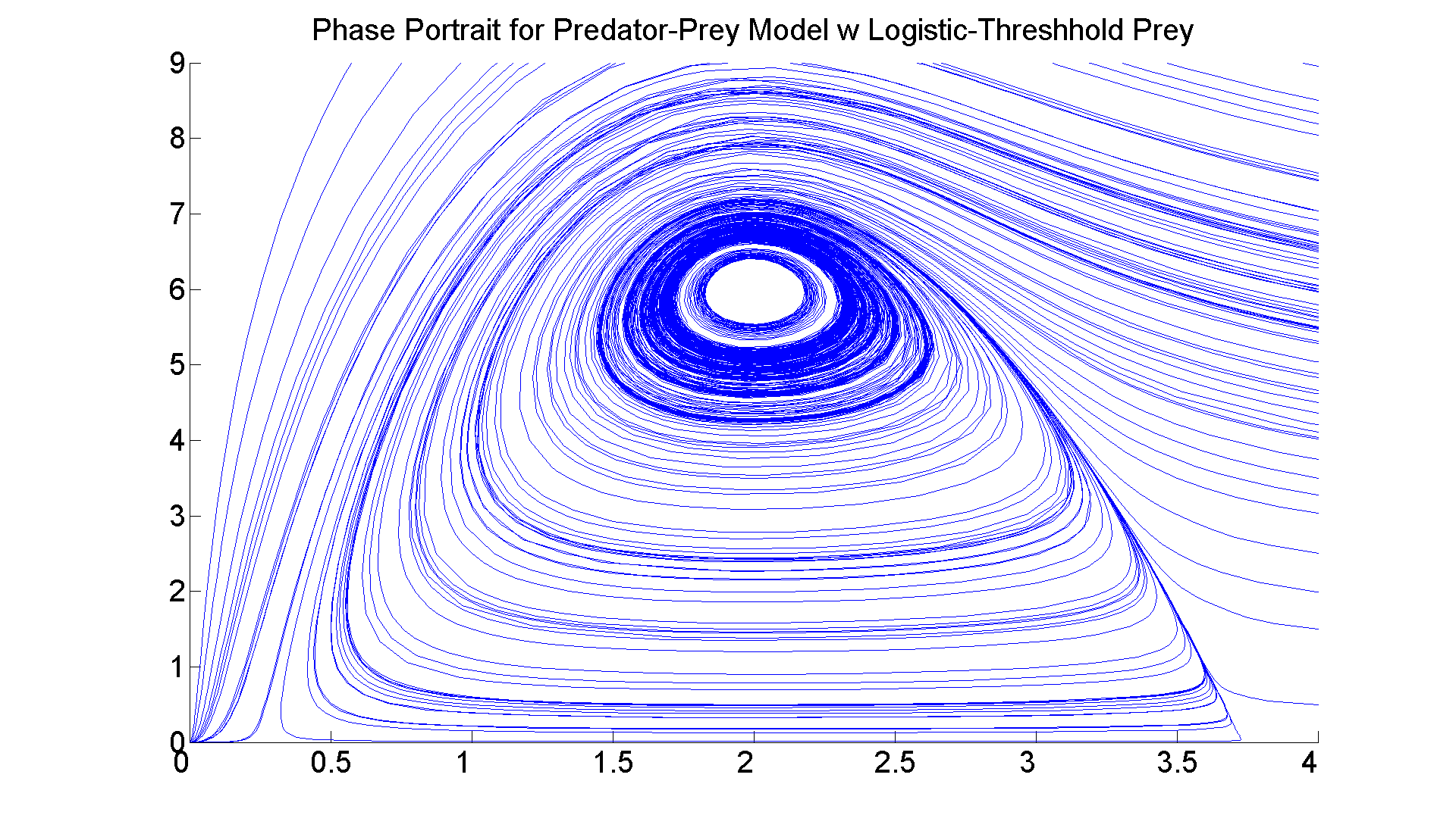
I leave it to you to think about the stability of the four critical points. Do you see them? What do you think?

% Just for fun, let's draw the separatrix:
hold on
[t, xa] = ode45(f, [0 -10], [2-sqrt(3) 0.01]);
plot(xa(:,1),xa(:,2), 'r', 'LineWidth', 2)
axis([0 4 0 9])
plot(0, 0, '*g', 'LineWidth', 10)
plot(2+sqrt(3),0,'*g', 'LineWidth', 10)
plot(2-sqrt(3),0,'*g', 'LineWidth', 10)
plot(2,6,'*g', 'LineWidth', 10)

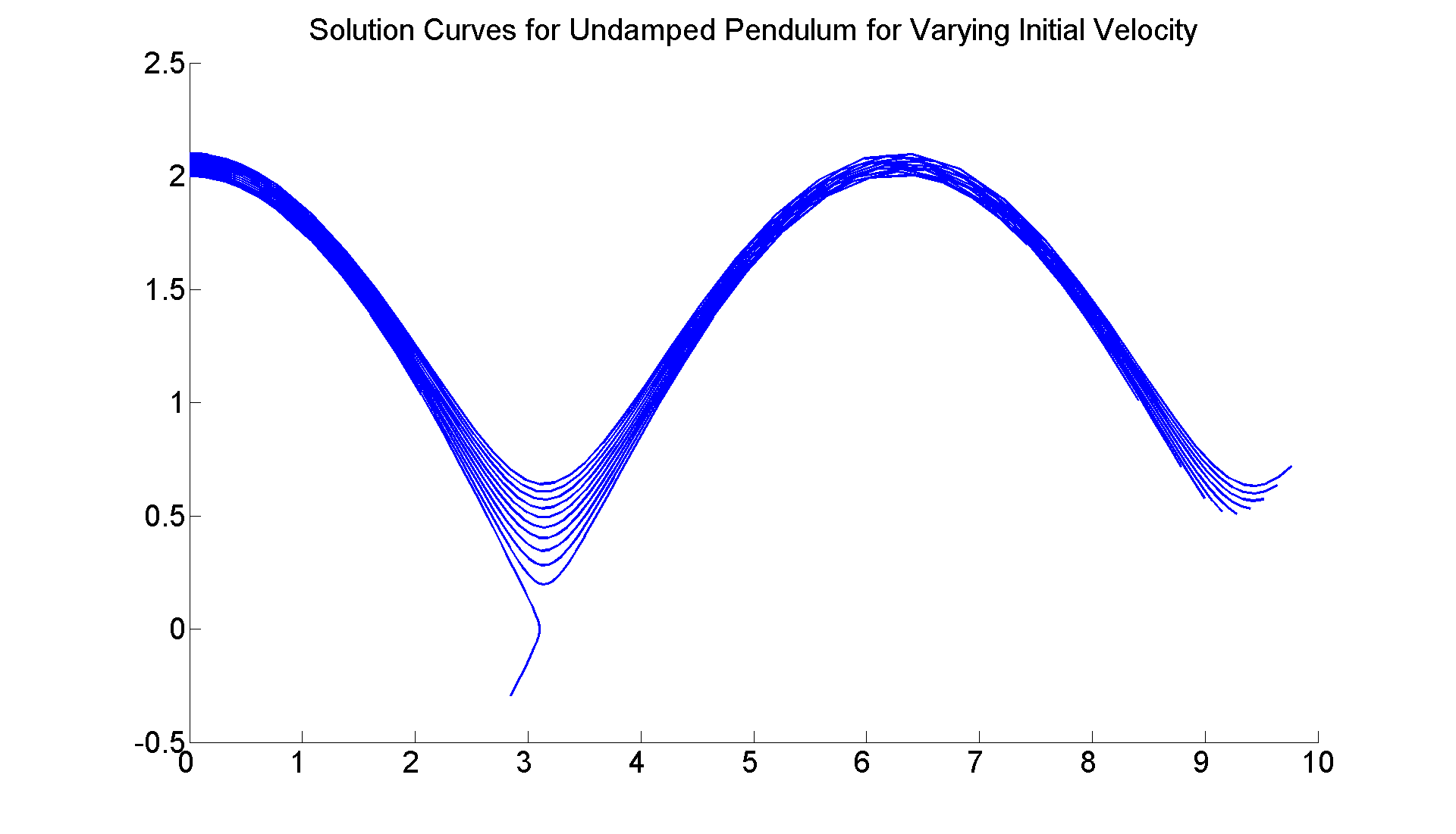
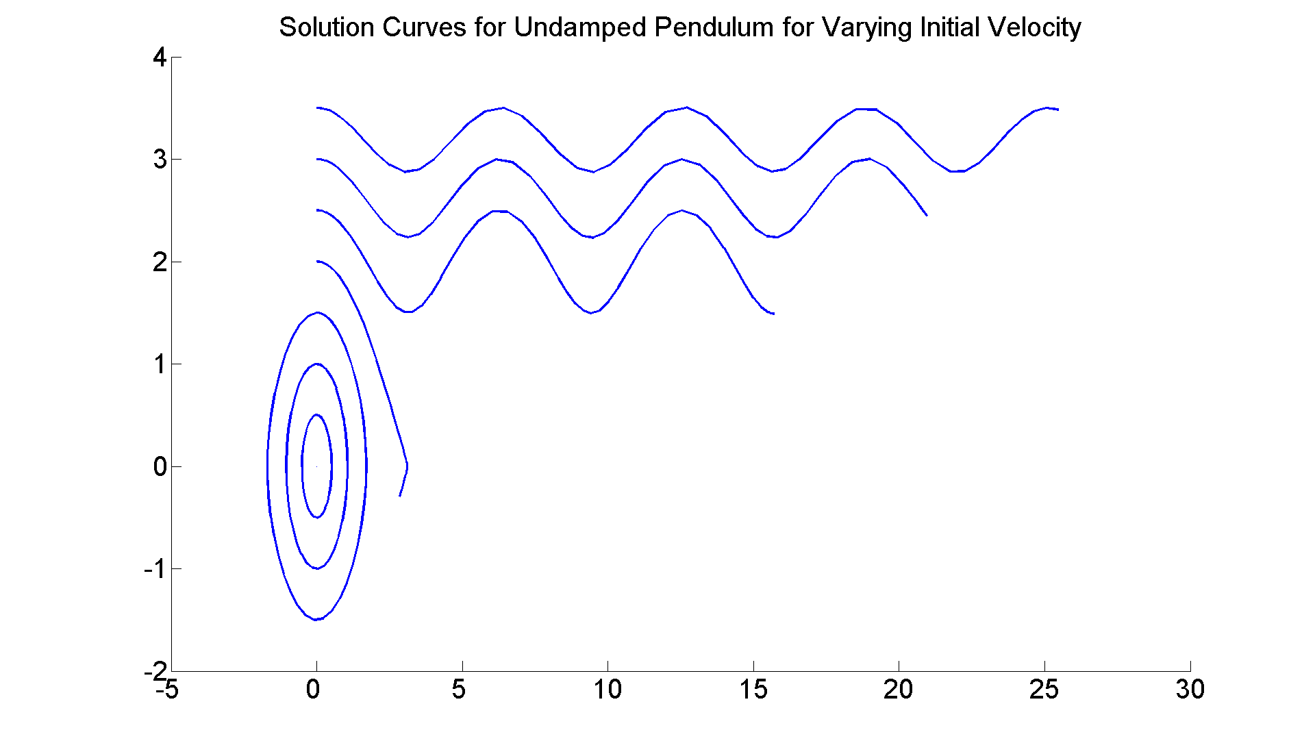
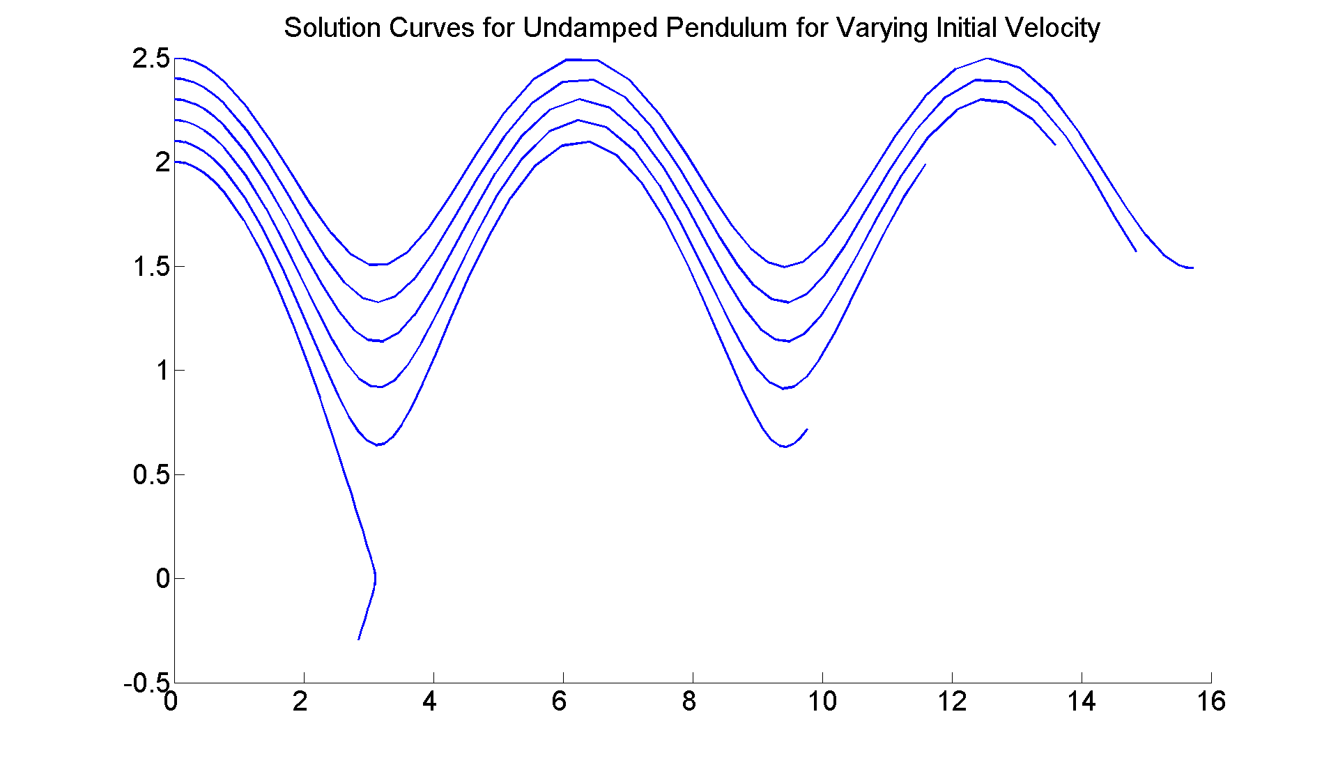
Finally, let's answer the question raised earlier about the undamped pendulum -- namely how hard do you have to hit it to make it rotate endlessly? I will graph numerically the solution curves corresponding to the pendulum starting in the vertical position but with harder and harder initial angular velocity; i.e., x(0) = 0, but y(0) = c, where I will increase c until the pendulum fails to fall back toward the vertical, but instead spins around ad infinitum.

figure; set(gcf, 'Position', [1 1 1920 1420])
axes; hold on
f = @(t, x) [x(2);-sin(x(1))];
for c=0:1/2:7/2
[t, xa] =ode45(f, [0 8], [0, c]);
plot(xa(:,1),xa(:,2), 'LineWidth', 2)
end
title ('Solution Curves for Undamped Pendulum for Varying Initial Velocity', 'FontSize', 25)
set(gca,'XTickLabel',get(gca, 'XTickLabel'),'FontSize',25)

% So the actual critical value is between 2 and 2.5. You can refine
% the search further by choosing initial velocities more finely,
% e.g., c =2: 0.1:2.5, and so on.

Exception in thread "AWT-EventQueue-0" java.lang.OutOfMemoryError: Java heap space

For example:

figure; set(gcf, 'Position', [1 1 1920 1420])
axes; hold on
f = @(t, x) [x(2);-sin(x(1))];
for c=2:0.1:2.5
[t, xa] =ode45(f, [0 8], [0, c]);
plot(xa(:,1),xa(:,2), 'LineWidth', 2)
end
title ('Solution Curves for Undamped Pendulum for Varying Initial Velocity', 'FontSize', 25)
set(gca,'XTickLabel',get(gca, 'XTickLabel'),'FontSize',25)

Exception in thread "AWT-EventQueue-0" java.lang.OutOfMemoryError: Java heap space

And then:

figure; set(gcf, 'Position', [1 1 1920 1420])
axes; hold on
f = @(t, x) [x(2);-sin(x(1))];
for c=2:0.01:2.1
[t, xa] =ode45(f, [0 8], [0, c]);
plot(xa(:,1),xa(:,2), 'LineWidth', 2)
end
title ('Solution Curves for Undamped Pendulum for Varying Initial Velocity', 'FontSize', 25)
set(gca,'XTickLabel',get(gca, 'XTickLabel'),'FontSize',25)

Exception in thread "AWT-EventQueue-0" java.lang.OutOfMemoryError: Java heap space