MATH/CMSC 206 - Introduction to Matlab

Announcements

Syllabus

Tutorial

Projects

Submitting

Limitations of Matlab

Contents

Understanding Matlab Commands

You should be aware that Matlab commands sometimes do what they do rather than what you might think they do. For example the fzero command doesn't really find a zero, rather it finds a place where the function crosses the x-axis. The reason is that fzero first finds an interval containing the seed value on which the function changes sign and then attempts to get close to this x-value. This means that if your function touches but does not cross the x-axis the interval won't be found and mayhem results. Try the following:

f=@(x) x^2;
fzero(f,1)

Exiting fzero: aborting search for an interval containing a sign change
    because NaN or Inf function value encountered during search.
(Function value at -1.7162e+154 is Inf.)
Check function or try again with a different starting value.

ans =

   NaN

You'll see the output is NaN, meaning Not a Number along with a warning that Matlab couldn't find a place where the function crosses the x-axis. Naturally, because it doesn't. Likewise fzero also finds discontinuities for somewhat similar reasons. For example:

fzero(@tan,1)

ans =

    1.5708

Tangent does not have a zero there, rather it has an asymptote.

The important thing is to make sure you understand what exactly each command does; use the help files and use your own intelligence to analyze and filter the results. In many cases a better command would be fsolve, which solves systems of nonlinear equations. The command is fsolve(function,seed value). The example with tangent above could instead be done as:

fsolve(@tan,1)

Optimization terminated: first-order optimality is less than options.TolFun.

ans =

   2.3205e-10

Which leads us to:

Precision Issues

Be aware that any Matlab command which uses approximation methods will yield an approximate result even if an exact result is obvious to us. We saw in our last example that our result is 2.3205x10^(-10). Of course the exact result should be 0. In this example though we're probably smart enough to say "Oh,that's pretty much 0 so we'll call it 0". However the problem becomes even more evident for the following example:

fsolve(@(x) x^2,1)

Optimization terminated: first-order optimality is less than options.TolFun.

ans =

    0.0078

Here again the answer should be 0 but we're way off! Even more annoying is that different seed values may give different answers:

fsolve(@(x) x^2,0.1)

Optimization terminated: first-order optimality is less than options.TolFun.

ans =

    0.0063

What's going on? The short answer is that Matlab is using an iterative method to find a root, meaning it gets closer and closer until it gets within a certain tolerance. What does this mean? Matlab's default tolerance is 1e-06 which means that the algorithm continues until an x-value arises such that the first-order optimality is within 1e-06. It's really important to understand this, that it's not the solution that's within the tolerance but the first-order optimality value.

As to what this first-order optimality actually means, this is not obvious. Suffice to say for now that the function is approximately within the tolerance from 0. That is, both 0.0078^2 and 0.0063^2 are very close to 0.

In the last two examples what's happened is that when the algorithm in the first case reaches 0.0078 and in the second case reaches 0.0063 the first-order optimality is within 1e-06 and the algorithm halts.

Just for fun, if you're interested, you can watch the algorithm work by adding an option:

fsolve(@(x) x^2,1,optimset('Display','Iter'))

                                         Norm of      First-order   Trust-region
 Iteration  Func-count     f(x)          step         optimality    radius
     0          2               1                             2               1
     1          4          0.0625            0.5           0.25               1
     2          6      0.00390625           0.25         0.0313            1.25
     3          8     0.000244141          0.125        0.00391            1.25
     4         10     1.52588e-05         0.0625       0.000488            1.25
     5         12     9.53675e-07        0.03125        6.1e-05            1.25
     6         14     5.96048e-08       0.015625       7.63e-06            1.25
     7         16      3.7253e-09      0.0078125       9.54e-07            1.25
Optimization terminated: first-order optimality is less than options.TolFun.

ans =

    0.0078

Which displays all the steps that Matlab goes through as it finds the answer.

Graphing

When we graph a function how exactly does Matlab do this? Matlab is not smart in that it doesn't know what functions look like nor does it do any analysis of a function when it graphs it. What Matlab does is it plots points and connects them with lines. There are two primary issues here.

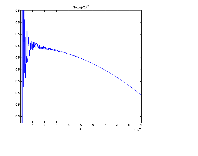
One issue is that precision issues arise when dealing with numbers very close to 0. This is true for computers in general, not just Matlab. For example consider the two functions y=(1-cos(x))/x^2 and y=sin(x)^2/(x^2*(1+cos(x))). Basic trigonometry shows that these functions are identical but look at the following two graphs:

ezplot(@(x) (1-cos(x))./x.^2,[10^-8,10^-3])

and then:

ezplot(@(x) sin(x).^2./(x.^2.*(1+cos(x))),[10^-8,10^-3])

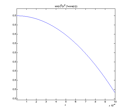
Wow! Look at the difference! What's going on?

The short answer is that for obscure computational reasons the first is mis-evaluating scores near 10^-8 whereas the second is not. One tip-off to this is the scale on the left which is completely composed of 0.5. Matlab is getting into trouble with y-values which are very close to on another. If you only looked at the first version you might be led to believe that the output oscillates near 10^-8 (it's got a cosine in it, why not?!) but this would be false.

This is not to say that we can tell you what to do to get the correct graph, just that you need to realize when to be careful - in this case when playing with values near 0. You know that for values of x near 0 cosine does not oscillate, it stays close to 1, hence this graph should not oscillate either.

Self-Test

syms x;
f=@(x) x^5-6*x^4+16*x^3-32*x^2+48*x-32;
fzero(inline(diff(f(x))),1)

Next Topic:   Introduction to MuPAD.

Published with MATLAB® 7.8